Introduction

Atwood (2022) (original code, my code) studies the long-term economic effects of the measles vaccine. Using US data and a difference-in-differences strategy, Atwood finds that the national rollout of the vaccine in 1963 increased earnings and employment for adults by preventing measles during childhood. The identification strategy interacts cross-sectional variation in pre-vaccine average reported measles incidence with time-series variation in the availability of the vaccine during childhood.

However, it is not clear how to interpret the geographic variation in pre-vaccine measles incidence, which is calculated as a state-level average over 1952-1963. Atwood notes that measles is a universal disease, with 95% of the population contracting the virus by age 16.¹ While states could differ in short-run measles incidence, due to staggered timing of the epidemic cycle, this variation would be averaged out over 12 years.² Hence, differences in reported incidence reflect differences in reporting rates, since actual long-run incidence is the same across states. Variation in reporting rates could be explained by differences in reporting capacity or differences in the impact of the disease. States could vary in their capacity to report cases of contagious diseases, if better health infrastructure enables the detection of a larger fraction of cases. Similarly, measles cases would be more severe in states with worse initial health, and more severe cases are more likely to be reported.

Atwood does not discuss reporting capacity or disease severity as sources of geographic variation in reported measles incidence,³ and instead attributes differences in measles incidence to under-18 population density. But the \(R^{2}\) from a cross-sectional regression of average reported measles incidence on under-18 population density is only 0.05 (Table A1, Atwood (2022)). Atwood claims that “states with higher prevaccine measles incidence benefited more from the introduction of the vaccine than states with lower levels of prevaccine measles incidence” (p.49). This claim is plausible if states with worse initial health have high reported incidence due to having more severe cases, and the vaccine has larger benefits for individuals with poor health.⁴ In contrast, if differences in reported incidence reflect reporting capacity, while actual disease incidence is the same, then it is not clear why states with higher reported incidence would benefit more from the vaccine.⁵

Since the identifying variation is ambiguous, we should be worried that differences between high- and low-measles states are capturing trends unrelated to the measles vaccine. In this comment, I replicate the main results using an expanded sample, and test for differential trends using an event study. The regression results are similar, but the event study shows post-vaccine trends that are inconsistent with a treatment effect of the vaccine.

Regression results

Atwood defines the treatment window (exposure to the vaccine) to be 16 years long, since measles incidence after age 16 is negligible. The treatment dose, vaccine exposure, is 0 for cohorts born in 1948 and earlier, increases by 1 per year until 1964, and is 16 for cohorts born afterwards.⁶ To test for trends before and after the vaccine, we want symmetric windows for 1932-1948 and 1964-1980. But Atwood uses 2000-2017 American Community Survey data on individuals aged 25-60, meaning the earliest cohort is 1940. To include cohorts from 1932-1939, I extend the sample using census data from 1960-1990.

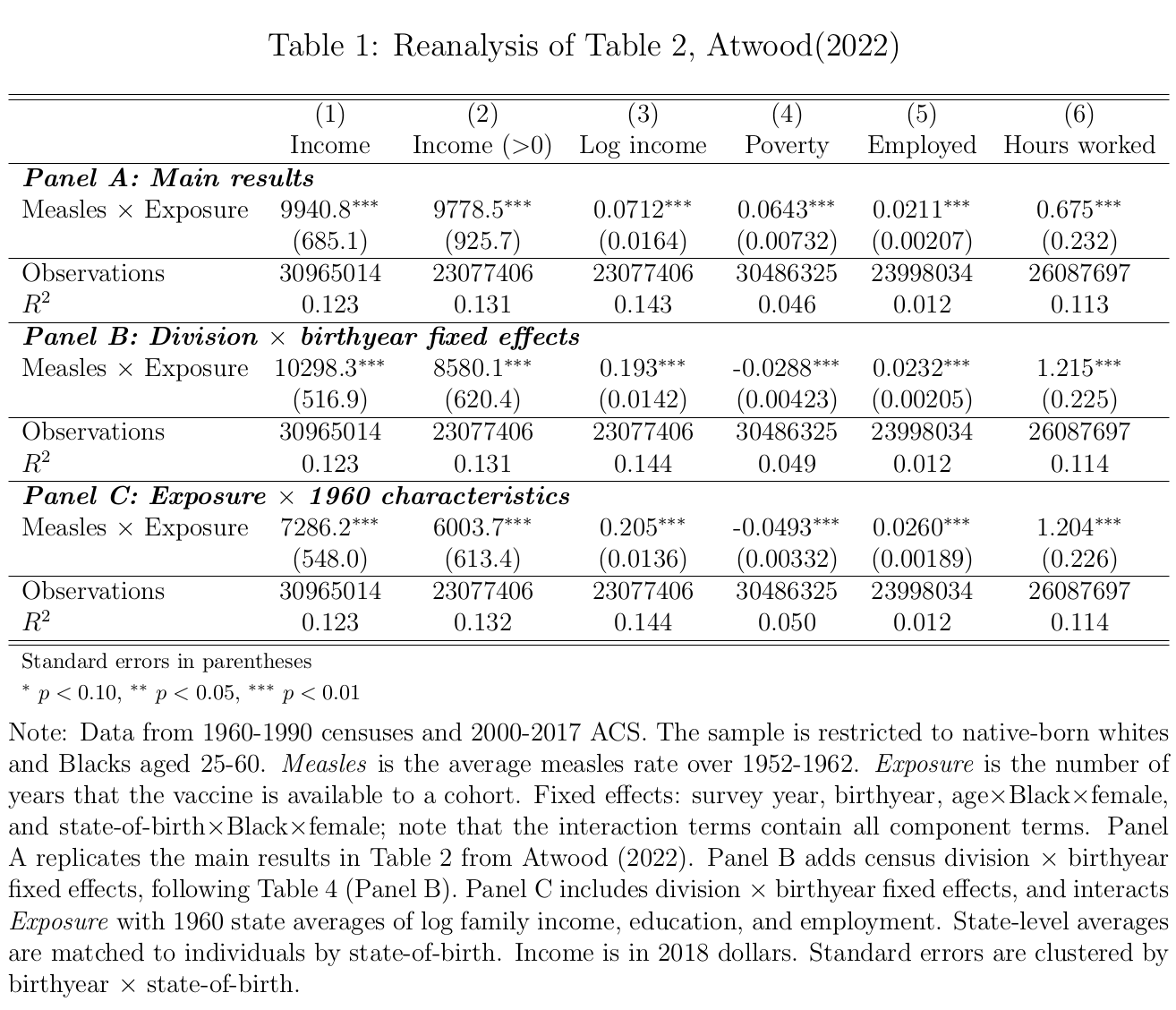
Atwood’s Table 2 estimates the long-run effects of childhood exposure to the measles vaccine on adult economic outcomes, using a difference-in-differences strategy with a continuous treatment variable. I replicate these results using the extended sample. The regression specification is

where \(y_{isct}\) is the outcome (income, poverty, employment, or hours worked) for individual \(i\) with state-of-birth \(s\) in birthyear \(c\), observed in survey year \(t\). Measles\(_{s}\) is the state-level average measles rate over 1952-1962⁷, and Exposure\(_{c}\) is the number of years that the vaccine is available to a cohort. Controls include fixed effects for survey year, birthyear, the interaction of age, Black, and female, and the interaction of state-of-birth, Black, and female.⁸ See the code snippet below.

* robustness: include region X birthyear FEs
use year sex age birthyr black bpl female cpi_incwage cpi_incwage_no0 ln_cpi_income poverty100 employed hrs_worked M12_exp_rate bpl_region9 exposure edu1960 employed1960 logfamincome1960 if missing(M12_exp_rate)==0 using "$data/acs_cleaned.dta", clear

local robust_fes year age#black#female bpl#black#female bpl_region9#birthyr

local i = 1

foreach x in cpi_incwage cpi_incwage_no0 ln_cpi_income poverty100 employed hrs_worked {

    reghdfe `x' M12_exp_rate, ab(`robust_fes') vce(cluster bpl#birthyr)
    est sto m`i'

    local i = `i' + 1
}

esttab m*, se label compress replace star(* 0.10 ** 0.05 *** 0.01) mtitles("Income" "Income ($>$0)" "Log income" "Poverty" "Employed" "Hours worked") nocons r2

My results are in Table 1. Panel A reproduces Table 2 using the extended sample. The results are similar to the original, except that the effects on poverty and hours worked are now positive instead of negative. In Panel B, I add fixed effects for census division by birthyear, to capture different trends across regions, following Table 4, Panel B in Atwood (2022). Now the effect on poverty has the expected negative sign, indicating that division-birthyear fixed effects are needed to control for trends when using the longer panel. The effect on hours worked is positive, matching Atwood’s Table 4. In Panel C, I additionally control for 1960 state-level averages of log family income, education, and employment interacted with vaccine exposure, following Bleakley (2007).⁹ The results are similar, showing that reported measles incidence captures variation separate from pre-vaccine state characteristics, conditional on the fixed effects.

Event study

To test for differential trends in the original results, I run an event study interacting pre-vaccine average reported measles incidence with birthyear indicators.¹⁰ The regression specification is

I restrict the sample to 1932-1980, to include symmetric pre- and post-periods matching the 16-year treatment window. See the code snippet below.

use year sex age birthyr black bpl female cpi_incwage cpi_incwage_no0 ln_cpi_income poverty100 employed hrs_worked avg_12yr_measles_rate bpl_region9 if inrange(birthyr,1932,1980) & missing(avg_12yr_measles_rate)==0 using "$data/acs_cleaned.dta", clear

gen measles_pc = avg_12yr_measles_rate/100000

forvalues i = 1932/1980 {
    gen d`i' = (birthyr==`i')
    gen int_`i' = d`i'*measles_pc
    lab var int_`i' " "
    drop d`i'
}

* loop to construct list by appending
    * put 1948 last, as omitted year
local interactions ""
forval y = 1932/1980 {
    if `y' != 1948 {
        local interactions "`interactions' int_`y'"
    }
}
local interactions "`interactions' int_1948"

local robust_fes year age#black#female bpl#black#female bpl_region9#birthyr

foreach x in cpi_incwage cpi_incwage_no0 ln_cpi_income poverty100 employed hrs_worked {
    reghdfe `x' `interactions', ab(`robust_fes') vce(cluster bpl#birthyr)
    coefplot, drop(_cons) vert omitted
}

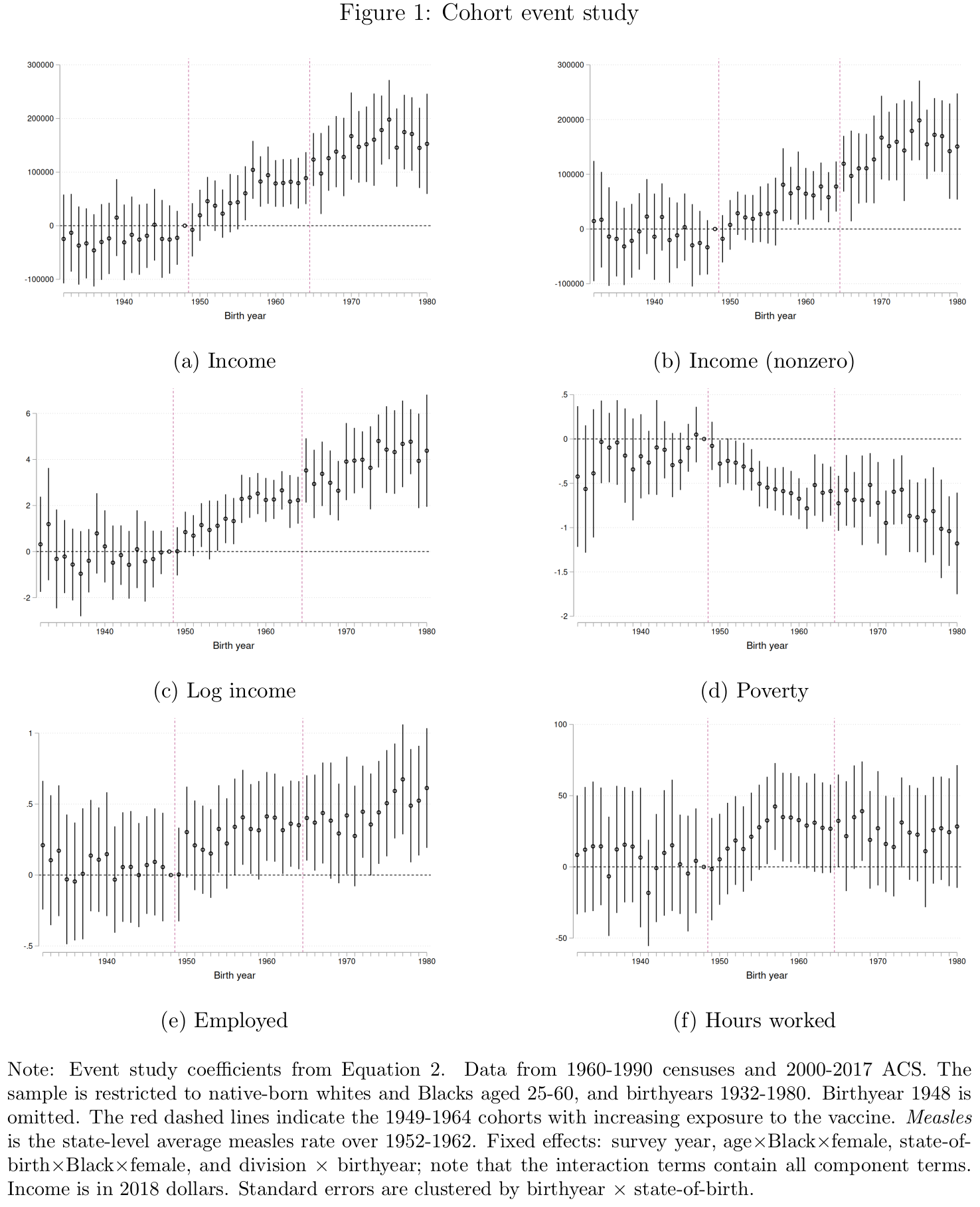
If the results in Table 1 are driven by the measles vaccine, we should observe the following: no trend in the event study coefficients before 1948, as all cohorts have equal access to the vaccine (that is, none); a trend in the coefficients from 1948-1964, as cohorts are increasingly exposed to the vaccine; and no trend for 1964-1980, when all cohorts again have equal access to the vaccine (that is, full access). In other words, the treatment effect should mirror the treatment dose.

The event study results are plotted in Figure 1. There is no evidence of trends in the coefficients before 1948. Moreover, the coefficients start to change in 1949, consistent with a treatment effect from the vaccine. However, for five of six outcomes, the coefficients continue to change after the vaccine was introduced in 1963. For example, in Panel (c), the coefficients for log income follow a rough positive trend from 1948 to 1980. This is inconsistent with a treatment effect of the vaccine, since there is no change in vaccine exposure between successive cohorts after 1963. That is, while the 1965 cohort benefits more from the vaccine than the 1955 cohort (because it is more likely that the former obtains immunity from the vaccine and avoids the health costs of measles), there is no such difference between the 1975 and 1965 cohorts.¹¹ Hence, the evidence in Atwood (2022) appears to reflect differential trends across states, rather than the effect of the measles vaccine.¹²

Conclusion

I reanalyze Atwood (2022) by extending the dataset and using an event study to test for differential trends. The identifying variation is from pre-vaccine average reported measles incidence, but for a contagious disease like measles, it is more plausible that this variation represents differences in reporting capacity or initial health levels than differences in actual disease incidence. The event study results for long-run economic outcomes show trends that are inconsistent with an effect of the vaccine.