I’ve seen a few papers that use randomization inference as a robustness check. They permute their treatment variable many times, and estimate their model for each permutation, producing a null distribution of estimates. From this null distribution we can calculate a randomization inference (RI) p-value as the fraction of estimates that are more extreme than the original estimate. (This works because under the null hypothesis of no treatment effect, switching a unit from the treatment to the control group has no effect on the outcome.) These papers show that RI p-values are similar to their conventional p-values, and conclude that their results are robust.

But robust to what, exactly?

Consider the case of using control variables as a robustness check. When adding control to a regression, we’re showing that our result is not driven by possible confounders. If the coefficient loses significance, we conclude that the original effect was spurious. But if the coefficient is stable and remains significant, then we conclude that the effect is not driven by confounding, and we say that it is robust to controls (at least, the ones we included).

Returning to randomization inference, suppose our result is significant using conventional p-values (\(p<0.05\)), but not with randomization inference (\(p_{RI}>0.05\)). What’s happening here? Young (2019) says that conventional p-values can have ‘size distortions’ when the sample size is small and treatment effects are heterogeneous, resulting in concentrated leverage. This means that the size, AKA the false positive rate \(P(\)reject \(H_{0} \mid H_{0}) = P(p<\alpha \mid H_{0})\), is higher than the nominal significance level \(\alpha\).¹ For instance, using \(\alpha =0.05\), we might have a false positive rate of \(0.1\). In this case, conventional p-values are invalid.

By comparison, RI has smaller size distortions. It performs better in settings of concentrated leverage, since it uses an exact test (with a known distribution for any sample size \(N\)), and hence doesn’t rely on convergence as \(N\) grows large. See Young (2019) for details. Upshot: we can think of RI as a robustness test for finite sample bias (in otherwise asymptotically correct variance estimates).

So in the case where we lose significance using RI (\(p<0.05\) and \(p_{RI}>0.05\)), we infer that the original result was driven by finite sample bias. In contrast, if \(p \approx p_{RI} <0.05\), then we conclude that the result is not driven by finite sample bias.

So RI is a useful robustness check for when we’re worried about finite sample bias. However, this is not the justification I’ve seen when papers use RI as a robustness check.

Randomization inference in Gavrilova et al. (2019)

This paper (published in Economic Journal) studies the effect of medical marijuana legalization on crime, finding that legalization decreases crime in states that border Mexico. The paper uses a triple-diff method, essentially doing a diff-in-diff for the effect of legalization on crime, then adding an interaction for being a border state.

Here’s how they describe their randomization inference exercise (p.24):

We run an in-space placebo test to test whether the control states form a valid counterfactual to the treatment states in the absence of treatment. In this placebo-test, we randomly reassign both the treatment and the border dummies to other states. We select at random four states that represent the placebo-border states. We then treat three of them in 1996, 2007 and 2010 respectively, coinciding with the actual treatment dates in California, Arizona and New Mexico. We also randomly reassign the inland treatment dummies and estimate [Equation] (1) with the placebo dummies rather than the actual dummies. [...]

If our treatment result is driven by strong heterogeneity in trends, the placebo treatments will often find an effect of similar magnitude and our baseline coefficient of -107.98 will be in the thick of the distribution of placebo-coefficients. On the other hand, if we are measuring an actual treatment effect, the baseline coefficient will be in the far left tail of the distribution of placebo-coefficients. [...]

Our baseline-treatment coefficient is in the bottom 3rd-percentile of the distribution. This result is consistent with a p-value of about 0.03 using a one-sided t-test.

At first glance, this reasoning seems plausible. I believed it when I first read this paper. The only problem is that it’s wrong.²

To prove this, I run a simulation with differential pre-trends (i.e., a violation of the common trends assumption). I simulate panel data for 50 states over 1995-2015 according to:

\[\tag{1} y_{st} = \beta D_{st} + \gamma_{s} + \gamma_{t} + \lambda \times D_{s} \times (t-1995) + \varepsilon_{st}.\]

Here \(D_{st}\) is a treatment dummy, equal to 1 in the years a state is treated. Ten states are treated, with treatment years selected randomly in 2000-2010; so this is a staggered rollout diff-in-diff. I draw state and year fixed effects separately from \(N(0,1)\). To generate a false positive, I set \(\beta=0\) and include a time trend only for the treatment group: \(\lambda \times D_{s} \times (t-1995)\), where \(\lambda\) is the value of the trend, and \(D_{s}\) is an ever-treated indicator.

Because the common trends assumption is not satisfied, diff-in-diff will wrongly estimate a significant treatment effect. According to Gavrilova et al., randomization inference will yield a large, nonsignificant p-value, since the placebo treatments will also pick up the differential trends and give similar estimates.

But this doesn’t happen. When I set a trend value of \(\lambda=0.1\), I get a significant diff-in-diff estimate 100% of the time, using both conventional and RI p-values. The actual coefficient is always in the tail of the randomization distribution, and not "in the thick" of it. The false positive is just as significant when using RI.

More generally, when varying the trend, I find that \(p \approx p_{RI}\). Figure 1 shows average rejection rates and p-values for the diff-in-diff estimate across 100 simulations, for different values of differential trends. We see that, on average, conventional and RI p-values are almost identical. As a result, the rejection rates are also similar.

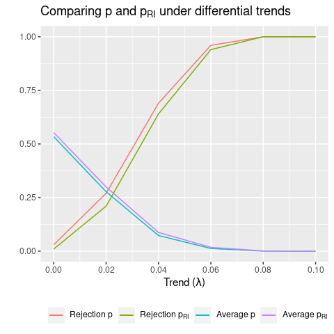
From the discussion above, we expect \(p_{RI}\) to differ when leverage is concentrated, due to small sample size and heterogeneous effects. Since this is not the case here, RI and conventional p-values are similar.

So Gavrilova et al.’s small randomization inference p-value does not prove that their result isn’t driven by differential pre-trends. False positives driven by differential trends also have small RI p-values. Randomization inference is a robustness check for finite sample bias, and nothing more.

---

Appendix: p-hacking simulations

Here I run simulations where I p-hack a significant result in different setups, to see whether randomization inference can kill a false positive. I calculate a RI p-value by reshuffling the treatment variable and calculating the t-statistic. I repeat this process 1000 times, and calculate \(p_{RI}\) as the fraction of randomized t-statistics that are larger (in absolute value) than the original t-statistic. According to Young (2019), using the t-statistic produces better performance than using the coefficient.

(1) Simple OLS

Constant effects: \(\beta=0\)

Data-generating process (DGP) with \(\beta=0\):

\[\tag{2} y_{i} = \sum_{k=1}^{K} \beta_{k} X_{k,i} + \varepsilon_{i} = \varepsilon_{i}\]

I p-hack a significant result by regressing \(y\) on \(X_{k}\) for \(k=1:K=20\), and selecting the \(X_{k}\) with the smallest p-value. I use \(N=1000\) and a significance level of \(\alpha=0.05\).

Running 1000 simulations, I find:

• An average rejection rate of 5.1% for the \(K=20\) regressions.

• 653 estimates (65%) are significant.³

• Out of these 653, 638 (98%) are significant using RI.

In this simple vanilla setup, RI and classical p-values are basically identical. So randomization inference is completely ineffective at killing false positives in a setting with large sample size and homogeneous effects.

Heterogeneous effects: \(\beta_{i} \sim N(0,1)\)

DGP with \(\beta_{k,i} \sim N(0,1)\):

\[\tag{3} y_{i} = \sum_{k=1}^{K} \beta_{k,i} X_{k,i} + \varepsilon_{i}\]

Again, I p-hack by cycling through the \(X_{k}\)’s and selecting the most significant one.

From 1000 simulations, I find:

• An average rejection rate of 5.2%.

• 645 estimates (65%) are significant.

• Out of these 645, 638 (99%) are significant using RI.

So even with heterogeneous effects, \(N=1000\) is enough to avoid finite sample bias, so RI p-values are no different.

(2) Difference in differences

Next I simulate panel data and estimate a diff-in-diff model as above, but with no differential trends.

Constant effects: \(\beta=0\)

DGP:

\[\tag{4} y_{st} = \beta D_{st} + \gamma_{s} + \gamma_{t} + \varepsilon_{st}\]

I simulate panel data for 50 states over 1995-2015. 10 states are treated, with treatment years selected randomly in 2000-2010; so this is a staggered rollout diff-in-diff. I draw state and year fixed effects separately from \(N(0,1)\). To generate a false positive, I set \(\beta=0\).

I p-hack a significant result by regressing \(y\) on K different treatment assignments \(D_{k,st}\) in a two-way fixed effects model, and selecting the regression with the smallest p-value. I cluster standard errors at the state level.

From 1000 simulations, I get

• An average rejection rate of 7.9%.

• 815 estimates (82%) are significant.

• Out of these 815, 653 (80%) are significant using RI.

So now we are seeing a size distortion using conventional p-values: out of the \(K=20\) regressions, 7.9% are significant, instead of the expected 5%. This appears to be driven by a small sample size and imbalanced treatment: 10 out of 50 states are treated. When I redo this exercise with \(N=500\) states and 250 treated, I get the expected 5% rejection rate.

However, RI doesn’t seem to be much of an improvement, as the majority of false positives remain significant using \(p_{RI}\).

Heterogeneous effects: \(\beta_{s} \sim N(0,1)\)

DGP:

\[\tag{5} y_{st} = \beta_{s} D_{st} + \gamma_{s} + \gamma_{t} + \varepsilon_{st}\]

Now I repeat the same exercise, but with the 10 treated states having treatment effects drawn from \(N(0,1)\).

From 1000 simulations, I get

• An average rejection rate of 7.7%.

• 790 estimates (79%) are significant.

• Out of these 790, 687 (87%) are significant using RI.

With heterogeneous effects as well as imbalanced treatment, RI performs even worse at killing the false positive.

What does it take to get \(p_{RI} \neq p\)?

I can get the RI p-value to differ by 0.1 (on average) when using \(N=20\), \(X \sim B(0.5)\), and \(\beta_{i} \sim\) lognormal\((0,2)\). So it takes a very small sample, highly heterogeneous treatment effects, and a binary treatment variable to generate a finite sample bias that is mitigated by randomization inference. Here’s a graph showing how \(|p-p_{RI}|\) varies with \(Var(\beta_{i})\):

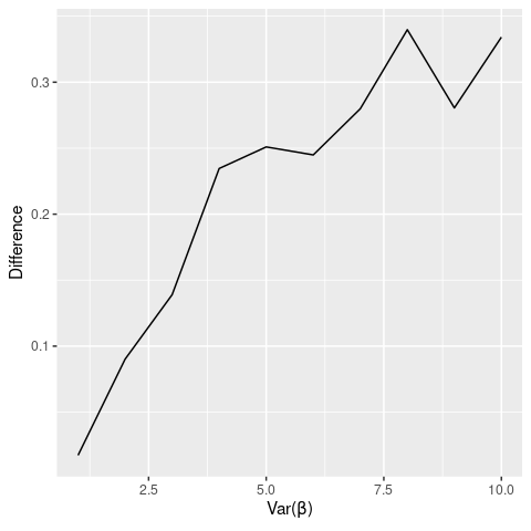
So it is possible for RI p-values to diverge substantially from conventional p-values, but it requires a pretty extreme scenario.

---

Footnotes

See here for R code.