How I use regression weights to replicate research

One of the main tools I use for replication is regression weights. These show the weight that each observation contributes to a regression coefficient. Suppose we’re regressing \(y\) on \(X_{1}\) and \(X_{2}\), with corresponding coefficients \(\beta_{1}\) and \(\beta_{2}\). Then, the regression weights for \(\beta_{1}\) are the residuals from regressing \(X_{1}\) on \(X_{2}\), which represent the variation in \(X_{1}\) remaining after controlling for \(X_{2}\). From Frisch-Waugh-Lovell, we know that \(\beta_{1}\) can be estimated by regressing \(y\) on these residuals. Hence, the regression weights show the actual variation used in the estimate. When replicating a paper, looking at regression weights is a handy way to see what’s actually driving the result.

In this post, I’ll give a quick demo of regression weights, looking at Cook (2014) (sci-hub) (replication files) on the effect of racial violence on African American patents over 1870-1940. This paper starts with striking time series data on patents by African American inventors. In Figure 1, we see a big drop in black patents around 1900. What is driving this pattern?

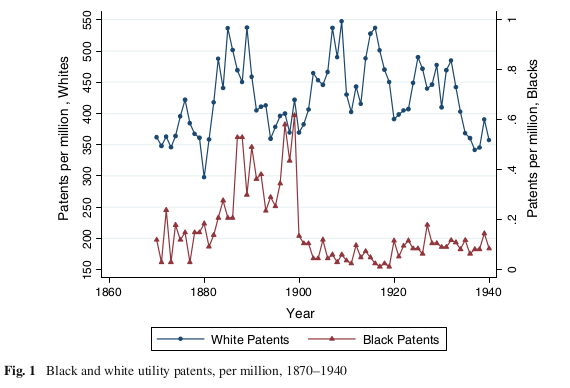
Cook argues that race riots and lynchings cause reduced patenting, directly by intimidating inventors, and indirectly by undermining trust in intellectual property laws (if the government won’t punish race rioters, why should you believe it’ll enforce your patents?).

Table 7 contains the main state-level regressions of patents on lynching rates and riots. Using a random-effects model, Cook finds negative effects for both lynchings and riots. I find similar results with a fixed effects model.

Let’s do regression weights, first for the lynching result. I regress lynchings on the other variables, grab the residuals, square them, then normalize by the sum of squared residuals.

* Stata code:

use pats_state_regs_AAonly, clear

reghdfe lynchrevpc riot seglaw illit blksh regs regmw regne regw , ab(stateno year1910 year1913 year1928) vce(cl stateno) res(resid)

gen res1 = resid^2
egen resid_tot = total(res1)
gen regweight = res1/resid_tot

Next, let’s see how these weights vary by region.

table region, c(sum regweight count patent)

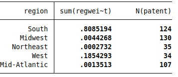
This is a bit surprising. The South has 81% of the weight, with the remainder coming from the West. The other three regions have basically zero contribution to the lynchings coefficient.

So let’s see what’s happening in the data.

table region, c(mean lynchrevpc)

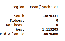
It turns out that basically all lynchings occurred in the South and West, with zero in the Midwest and Northeast (and roughly zero in Mid-Atlantic). Given this, the regression weights make sense. When there’s no variation in a variable, it should contribute nothing to the regression. But because the Midwest and Northeast have data on the other covariates, they still add some information, which is why the weights aren’t exactly zero.

Next, let’s see the results for the effect of riots on patenting. First, the regression weights, regressing riots on the other controls:

reghdfe riot lynchrevpc seglaw illit blksh regs regmw regne regw , ab(stateno year1910 year1913 year1928) vce(cl stateno) res(resid2)

gen res2 = resid2^2
egen resid_tot2 = total(res2)
gen regweight2 = res2/resid_tot2

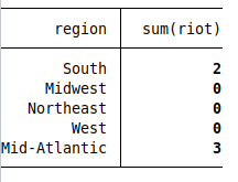
table region, c(sum regweight2 count patent)

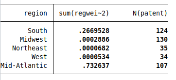
Again, the regional patterns are surprising. This time, the South has 27% of the weight, and the Mid-Atlantic has 73%, with the other regions contributing nothing. What’s going on?

gen region = .
replace region = 1 if (regs)
replace region = 2 if (regmw)
replace region = 3 if (regne)
replace region = 4 if (regw)
replace region = 5 if (regmatl)

label define reg_label 1 "South" 2 "Midwest" 3 "Northeast" 4 "West" 5 "Mid-Atlantic"
label values region reg_label

table region, c(sum riot)

It turns out there are only 5 riots in the state-level data. Let’s dig deeper.

table stateno, c(sum regweight2 count patent)
table year, c(sum regweight2 count patent)

* output omitted

The regression weight is concentrated on three states: state 39 has 58%, state 44 has 27%, and state 33 has 15% (the names are not in the data). It’s also concentrated on four years: 56% on 1917, 12% on 1918, 15% on 1900, 12% on 1906. This is because there are five riots occurring in four years, with two in 1917 in state 39, two in state 44 in different years, and one in state 33. So the riot effect is driven almost entirely by the four state-year observations that had riots.

But wait. If you look, you’ll see that there are 35 riots in the time-series data.

use pats_time_series, clear
collapse (sum) riot if race==0
su riot

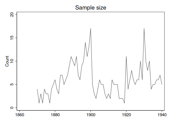
Where did the other riots go? It looks like the state data just has a lot of missing observations, which would explain the missing riots. That is, the issue isn’t variables with missing values, but that most state-year observations do not even have a row in the data. (I emailed Cook to ask about this, but didn’t get a response.) As you can see, the sample size fluctuates over time; this is far from a balanced panel.

Note that 1917 and 1918 have the majority of the weight, but there are only two observations in each of those years.

The paper is not very clear about this. Table 5 reports the descriptive stats, but only has the riots variable for the time-series data, and not the state-level data. And Cook does not plot any of the raw state-level data, but instead jumps right into the regressions.

This seems like a serious problem for the riot results. The paper isn’t estimating the effect of riots on patenting; instead, it’s doing the effect of five specific riots. If we could collect data on the remaining 30 riots, I’d expect the estimate to change. In other words, why should we expect this result to be externally valid for other historical riots?

To sum up, regression weights are an easy way to dig into a paper and see exactly what’s driving their results.

Happy replicating!