When we build new apartments, the people moving in vacate their old apartments; this reduces competition for old housing, making it more affordable. This is the vacancy chain effect: building expensive new housing helps improve affordability of cheaper old housing.

When rich people move into a city, they outcompete locals for new homes; those locals in turn compete for the stock of old homes, raising prices for poor people. This demand cascade is the mechanism driving the housing crisis. We can reverse demand cascades by building yuppie fishtanks to absorb the demand of rich newcomers.

In this post I’ll show how to use supply and demand to model vacancy chains, demand cascades, and yuppie fishtanks. I explain how to formalize the key mechanism in these scenarios, where changes to one market have effects on another market. This post treats quantity as continuous (so people can demand 1.26 homes, say) to show how standard microeconomics applies to housing; a future post will consider discrete quantity and unit demand.

A supply and demand equilibrium

Let’s consider an example of n=3 consumers with perfect substitutes preferences. People choose between Old and New apartments, and have a housing budget to spend. They differ in how much they prefer New vs Old apartments, and in the size of their housing budget. With perfect substitutes, you choose one good or the another, and spend your entire budget on the chosen good. For example, Person 1 will buy Old if price(Old) is less than half of price(New). Conversely, they buy New if price(New) is less than double price(Old). (We use two housing types as the simplest model that demonstrates the key mechanism; in reality, there are dozens of quality gradations.)

Here are the individual demand curves for Old apartments. Preference for Old (vs New) is decreasing from Person 1 to Person 3 (since Person 1 chooses an Old apartment at the highest price) while budget size is increasing (at price=2, Person 3 demands the largest quantity). Since New apartments are better, everyone gets more utility from a New apartment compared to an Old one, but they differ in how much more.

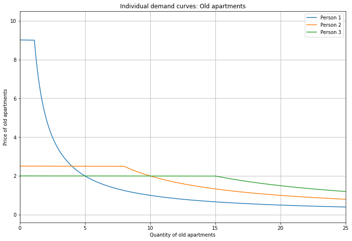
People choose between Old and New apartments based on a threshold determined by their preferences and the ratio of prices of Old and New apartments. Demand for Old apartments is equal to 0 above the threshold (here the demand curve overlaps the y-axis), is indeterminate at the threshold (the horizontal segment), and is equal to budget divided by price below the threshold (recall the shape of a 1/x function). Technically, the demand function has a discontinuity at the threshold, so you can imagine the horizontal part as being a dotted line. Also note that I’m referring to quantity demanded as a function of price, even though price is on the y-axis. Here I’m following the convention to plot price against quantity.

For example, Person 1 (blue) buys an Old apartment when the price is less than 9. Their quantity demanded is equal to their income (10) divided by the price; at price=2, this is 10/2=5. When the price is above 9, they demand 0 Old apartments and instead choose a New apartment; we’ll see that when we plot the demand curves for New apartments. When the price is equal to 9, their demand curve has a discontinuity and jumps across the horizontal segment.

Note that demand for Old apartments is a function of the prices of both Old and New apartments, but I’ve plotted it using only price(Old). What’s going on? The short answer is that I’m showing you one slice of the entire demand function, evaluated at a particular value of price(New). I’ll return to this later on.

Click below to see the underlying demand functions.

Math

Let \(x_{1}\) = Old apartments, \(x_{2}\) = New apartments. Let \(x_{i,j}\) be quantity demanded for consumer \(i\) of good \(j\), with income \(m_{i}\). Given perfect substitutes utility \(u(x_{1},x_{2}) = a x_{1} + b x_{2}\), we can derive the demand functions with the threshold defined by equating the marginal rate of substitution (\(a/b\)) with the price ratio (\(p_{1}/p_{2}\)). If \(p_{1}/a > p_{2}/b\), the consumer chooses \(x_{1}\) and spends their entire budget on it; otherwise, they choose \(x_{2}\). With perfect substitutes preferences, we get a corner solution: the optimal choice is one or the other, and not a mix of both. Note that the demand functions take both \(p_{1}\) and \(p_{2}\) as arguments, so they define a 3-dimensional surface. I use supply functions \(S_{1}(p_{1}) = 13\) (perfectly inelastic supply) and \(S_{2}(p_{2}) = \frac{3}{10} p_{2}\). \(S_{2}\) shifts to \(S_{2}^{new}(p_{2}) = \frac{50}{9} p_{2}\).

\[\begin{aligned} \begin{split} &u_{1}(x_{1},x_{2}) = 9x_{1} + 10x_{2} \\ &u_{2}(x_{1},x_{2}) = x_{1} + 4x_{2} \\ &u_{3}(x_{1},x_{2}) = x_{1} + 5x_{2} \\ &m_{1} = 10 \\ &m_{2} = 20 \\ &m_{3} = 30 \\ % \end{split} % \end{aligned} % \begin{aligned} % \begin{split} &x_{1,1} = \bigg\{ \begin{matrix} 0, p_{1} > \frac{9p_{2}}{10} \\ \frac{m_{1}}{p_{1}}, p_{1} \leq \frac{9p_{2}}{10} \\ \end{matrix} \\ &x_{1,2} = \bigg\{ \begin{matrix} \frac{m_{1}}{p_{2}}, p_{1} > \frac{9p_{2}}{10} \\ 0, p_{1} \leq \frac{9p_{2}}{10} \\ \end{matrix} \\ &x_{2,1} = \bigg\{ \begin{matrix} 0, p_{1} > \frac{p_{2}}{4} \\ \frac{m_{2}}{p_{1}}, p_{1} \leq \frac{p_{2}}{4} \\ \end{matrix} \\ &x_{2,2} = \bigg\{ \begin{matrix} \frac{m_{2}}{p_{2}}, p_{1} > \frac{p_{2}}{4} \\ 0, p_{1} \leq \frac{p_{2}}{4} \\ \end{matrix} \\ &x_{3,1} = \bigg\{ \begin{matrix} 0, p_{1} > \frac{p_{2}}{5} \\ \frac{m_{3}}{p_{1}}, p_{1} \leq \frac{p_{2}}{5} \\ \end{matrix} \\ &x_{3,2} = \bigg\{ \begin{matrix} \frac{m_{3}}{p_{2}}, p_{1} > \frac{p_{2}}{5} \\ 0, p_{1} \leq \frac{p_{2}}{5} \end{matrix} \\ \end{split} \end{aligned}\]

What does it mean to demand multiple apartments? A more complicated model would have unit-demand (ie. people demand either one Old or one New apartment), but it’s simpler to use continuous quantity to start. For now, you can interpret it as the square footage of the apartment, which is a continuous variable.

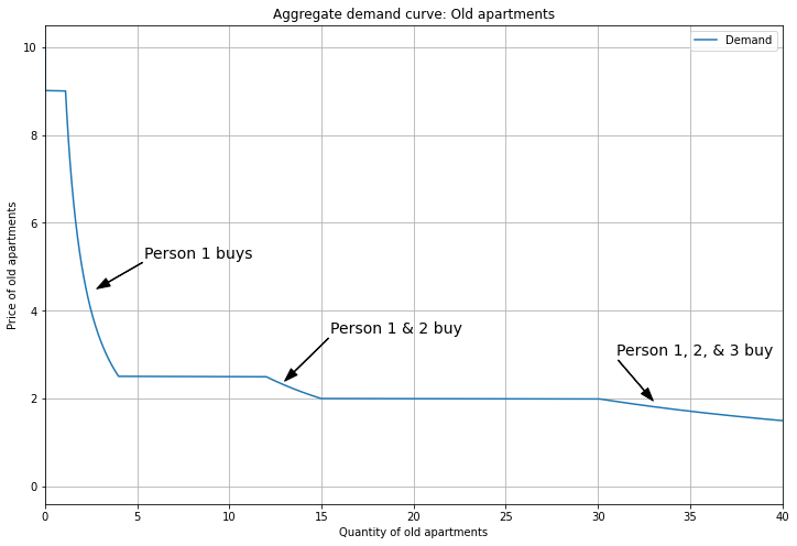
We get aggregate demand by summing up the individual demand curves: for each price, count the quantity demanded across consumers. This produces downward-sloping segments where we can identify which consumers contribute to aggregate demand. (Recall that the horizontal segments are discontinuities, so I have the arrows pointing at the sloped portions of the curve.) Since Person 1 has the strongest preference for Old apartments, they show up at the top of the demand curve, while Person 3 (with the weakest preference) shows up only at the bottom.

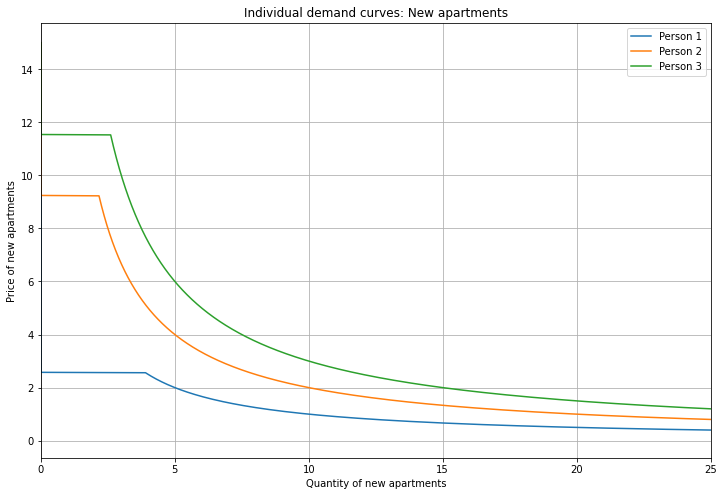
Next, let’s see the individual demand curves for New apartments. These are the reverse of demand for Old: because Person 1 had the strongest preference for Old (vs New), they have the weakest preference for New (vs Old). Again, budget size is increasing from Person 1 to 3. And keep in mind that these demand curves are evaluated at a specific value of price(Old).

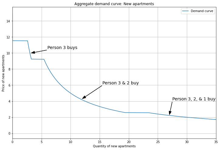
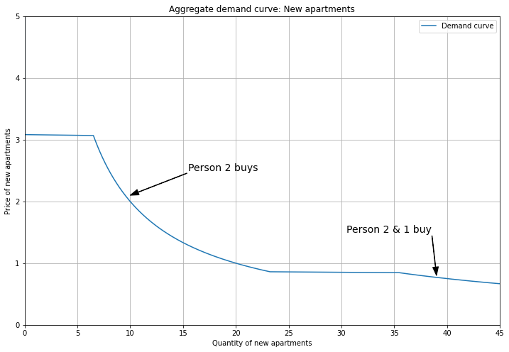
Here’s aggregate demand for New apartments. Now Person 3 has the strongest preference, so they contribute to aggregate demand in all segments, while Person 1 contributes only in the bottom segment.

An equilibrium is prices \((P_{Old}, P_{New})\) that set quantity supplied equal to aggregate quantity demanded in both markets. This is where the demand curve being evaluated at the price of the other good is key: the equilibrium price in one market has to be consistent with the equilibrium price in the other. I’ll show an equilibrium where Person 2 initially buys an Old apartment. To capture the vacancy chain effect, we’ll increase supply of New apartments, lowering the price, which induces Person 2 to upgrade from Old to New and reduces demand for Old apartments, thereby reducing pressure in that market.

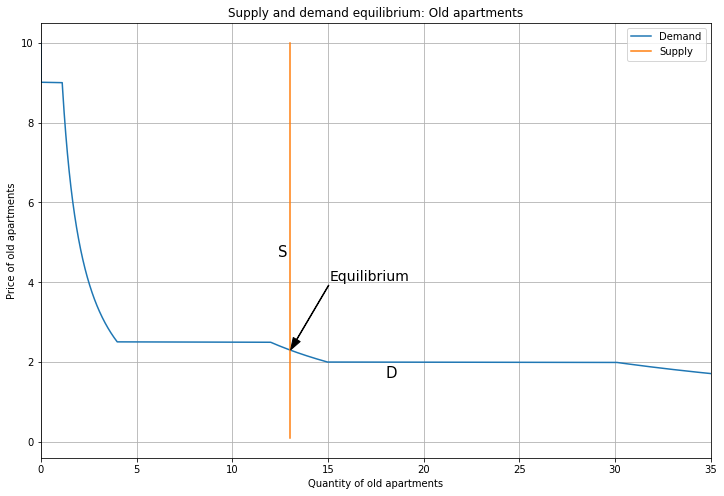
Here’s an equilibrium for Old apartments. To capture the stock of Old apartments being fixed, I use a vertical supply curve; no matter what the price is, developers can’t add any more old apartments (at least in the short run). I’ve chosen the supply curve so that Person 1 & 2 buy Old, while Person 3 buys New (ie. we’re on the second segment of the demand curve for Old apartments). The price is set by the intersection of the supply and demand curves; here, \(P_{Old} = 2.3\).

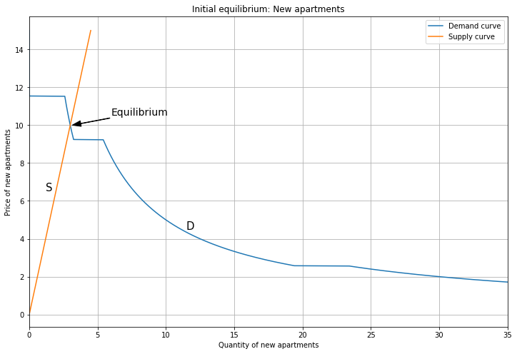
Here’s the corresponding equilibrium for New apartments. In this case, the supply curve is upward sloping, reflecting that developers are willing to build more units at higher prices (and that building them is permitted by zoning, which may be an unrealistic assumption). Supply intersects demand on the segment of the demand curve where only Person 3 buys a New apartment. Here the price is \(P_{New} = 10\).

You can confirm that these prices are the ones I used when plotting the demand curves for the other good. For example, the first graph shows the individual demand curves for Old apartments when price(New) = 10.

When a consumer buys one good, what happens to their demand for the other one? With perfect substitutes preferences, the demand is still there, but it can never be realized, because perfect substitutes involves a knife-edge threshold. For Person 2, if price(Old) \(<\) price(New)/4, they buy Old; otherwise they buy New. Here, that is 2.3 \(<\) 10/4 = 2.5, hence they buy Old. If the prices were different in a way that flipped the inequality, they would buy New. (But to be an equilibrium, the supply curve would have to match the quantity demanded.) In the next post on unit demand, I’ll show how this logic changes.

Stepping back, note that these demand functions are actually 2D slices of a 3D demand surface. Demand for Old apartments depends on the prices of both Old and New apartments, so it makes sense that the demand curve will be plotted as a function of two variables (the two prices). Here’s a plot of an individual demand surface (for Old apartments). The demand curves plotted above are slices of this surface, taken at specific values of price(New). If you rotate your head to the left, you can see it: when price(Old) is high, demand is 0 (overlapping the y-axis); the original horizontal discontinuity becomes vertical here in 3D; and as price(Old) goes to 0, quantity becomes large, following the 1/x shape.

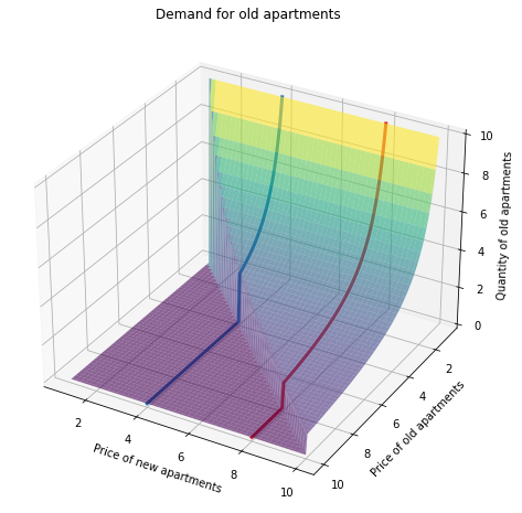
Changing the price of the other good moves you along the surface, but in 2D this will look like shifting the demand curve. This is important, because changing the cross-price does not shift demand in the sense of changing preferences. Instead, we’re evaluating the same demand function at a different price. For example, moving from price(New)=8 to price(New)=4 does not represent a change in preferences, but the demand curves (evaluated as slices at those prices) will look different, reflecting different tradeoffs (i.e., as New apartments get cheaper, my demand for Old apartments falls).

Vacancy chains

Let’s see how a vacancy chain works. The idea is that building new apartments will induce people to upgrade from Old to New, thereby reducing demand for Old apartments and making them more affordable.

We start the chain by increasing the supply of new apartments. For example, upzoning reduces land costs, which makes developers willing to produce more at every price. Shifting from S1 to S2, we move down the demand curve, with a new price \(P_{New}=3\).

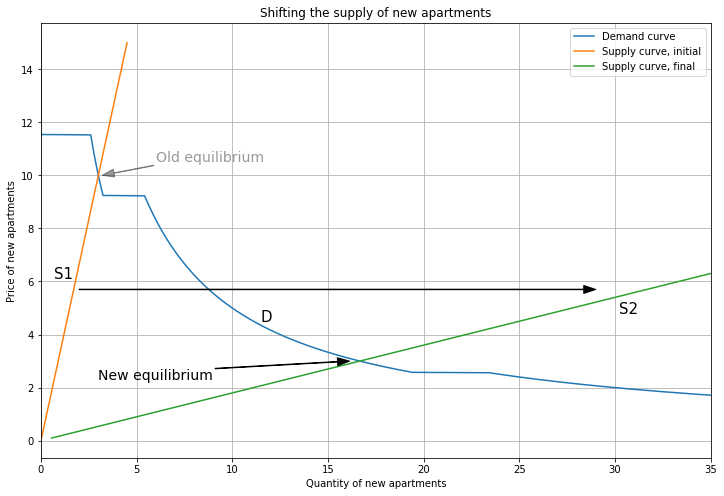
Note that now supply intersects demand in the segment where both Person 3 and 2 buy New. Induced by the lower price of New apartments (\(P_{New}\) falls from 10 to 3), Person 2 has upgraded from Old to New! So we should see a corresponding drop in demand for Old apartments.

Here’s the effect on Old apartments. The demand curve ‘shifts’ down from D1 to D2, and now supply intersects demand on the segment where only Person 1 buys Old. The price falls from \(P_{Old}=2.3\) to \(P_{Old}=0.8\). Following the intuition for subsitute goods, when price(New) falls, Old apartments become relatively less attractive, so demand for Old apartments decreases.

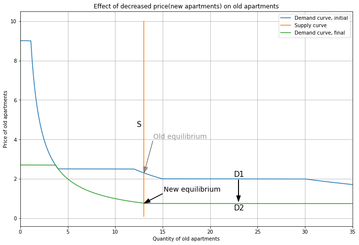
As mentioned above, this is not really a shift in demand, but a movement along the 3D demand surface caused by changing price(New). Person 2’s preferences haven’t changed, they just make a different choice at a different price.

So we’ve shown the vacancy chain effect: increasing the supply of new apartments reduces their price (from 10 to 3), which induces people to upgrade from old to new apartments, thereby reducing demand for and the price of old apartments (from 2.3 to 0.8). Thanks to the new apartments being built, Person 1 now gets all 13 of the Old units to themself, and at a lower price.

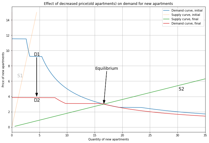
But if price(Old) fell, shouldn’t that reduce demand for New apartments too? Yes. These are substitute goods, so a reduction in the other price makes a good less appealing. In this case, demand for New apartments ‘shifts’ down, but not enough to change the equilibrium. Hence, there are no more changes, and we’ve converged on a new equilibrium, with \((P_{Old}, P_{New})\) = (0.8, 3).

If we added more consumers, we could show how the vacancy chain allows a poorer person to afford an Old apartment at the new lower price, when they were originally priced out. And with more housing sub-markets (with multiple degrees of quality, instead of only Old vs New), we could trace out the vacancy chain itself, with someone upgrading in each submarket and reducing demand for their original housing type, thereby enabling someone in the submarket below to upgrade.

Demand cascades and yuppie fishtanks

Now let’s look at demand cascades and yuppie fishtanks. When rich people move into the city, they increase demand for expensive new apartments. This pushes locals to downgrade, increasing demand for old apartments. The end result is higher prices for both old and new housing; sound familiar?

But when we increase the supply of new apartments to match the rise in demand, we can prevent the demand cascade and stop the price of old apartments from going up. This is a yuppie fishtank, where we build shiny glass towers to contain the rich yuppies moving in and absorb their demand for housing.

To illustrate, I’ll show an example with two people forming an initial equilibrium, which is disrupted by a rich person moving in.

Click below to see the underlying demand functions.

Math

Let \(x_{1}\) = Old apartments, \(x_{2}\) = New apartments. Let \(x_{i,j}\) be quantity demanded for consumer \(i\) of good \(j\), with income \(m_{i}\). Given perfect substitutes utility \(u(x_{1},x_{2}) = a x_{1} + b x_{2}\), we can derive the demand functions with the threshold defined by equating the marginal rate of substitution (\(a/b\)) with the price ratio (\(p_{1}/p_{2}\)). If \(p_{1}/a > p_{2}/b\), the consumer chooses \(x_{1}\) and spends their entire budget on it; otherwise, they choose \(x_{2}\). With perfect substitutes preferences, we get a corner solution: the optimal choice is one or the other, and not a mix of both. Note that the demand functions take both \(p_{1}\) and \(p_{2}\) as arguments, so they define a 3-dimensional surface. I use supply functions \(S_{1}(p_{1}) = 13\) (perfectly inelastic supply) and \(S_{2}(p_{2}) = \frac{20}{21} + \frac{41}{21} p_{2}\). \(S_{2}\) shifts to \(S_{2}^{new}(p_{2}) = \frac{20}{21} + \frac{1520}{63} p_{2}\).

\[\begin{aligned} \begin{split} &u_{1}(x_{1},x_{2}) = 9x_{1} + 10x_{2} \\ &u_{2}(x_{1},x_{2}) = x_{1} + 4x_{2} \\ &u_{3}(x_{1},x_{2}) = x_{1} + 15.6x_{2} \\ &m_{1} = 10 \\ &m_{2} = 20 \\ &m_{3} = 200 \\ % \end{split} % \end{aligned} % \begin{aligned} % \begin{split} &x_{1,1} = \bigg\{ \begin{matrix} 0, p_{1} > \frac{9p_{2}}{10} \\ \frac{m_{1}}{p_{1}}, p_{1} \leq \frac{9p_{2}}{10} \\ \end{matrix} \\ &x_{1,2} = \bigg\{ \begin{matrix} \frac{m_{1}}{p_{2}}, p_{1} > \frac{9p_{2}}{10} \\ 0, p_{1} \leq \frac{9p_{2}}{10} \\ \end{matrix} \\ &x_{2,1} = \bigg\{ \begin{matrix} 0, p_{1} > \frac{p_{2}}{4} \\ \frac{m_{2}}{p_{1}}, p_{1} \leq \frac{p_{2}}{4} \\ \end{matrix} \\ &x_{2,2} = \bigg\{ \begin{matrix} \frac{m_{2}}{p_{2}}, p_{1} > \frac{p_{2}}{4} \\ 0, p_{1} \leq \frac{p_{2}}{4} \\ \end{matrix} \\ &x_{3,1} = \bigg\{ \begin{matrix} 0, p_{1} > \frac{p_{2}}{15.6} \\ \frac{m_{3}}{p_{1}}, p_{1} \leq \frac{p_{2}}{15.6} \\ \end{matrix} \\ &x_{3,2} = \bigg\{ \begin{matrix} \frac{m_{3}}{p_{2}}, p_{1} > \frac{p_{2}}{15.6} \\ 0, p_{1} \leq \frac{p_{2}}{15.6} \end{matrix} \\ \end{split} \end{aligned}\]

Here are Person 1 and Person 2’s demand curves for Old apartments. As before, Person 1 has a stronger preference for Old apartments (relative to Person 2), and Person 2 has a larger budget.

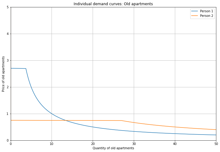
We sum their demand curves to get aggregate demand.

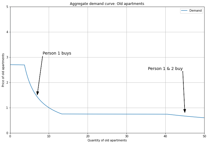
Now let’s see the demand curves for New apartments. In this case, Person 3 is much richer and has a very strong preference for New apartments.

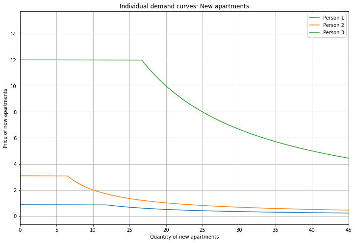
But they will move in later, so the aggregate demand curve does not include them (yet).

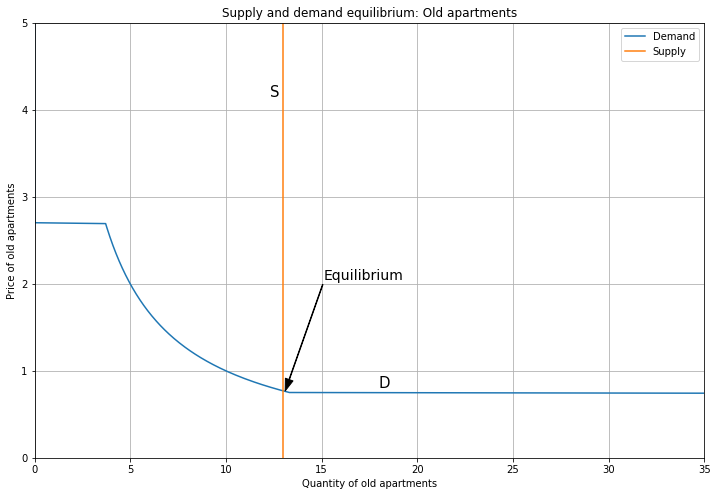
Here’s the initial equilibrium for Old apartments. Supply intersects demand on the segment where only Person 1 buys. The price is \(P_{Old} = 0.8\). As before, the supply curve is vertical, representing a fixed stock of Old apartments.

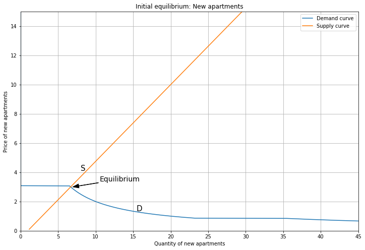
And here’s the initial equilibrium for New apartments. Supply intersects demand on the segment where only Person 2 buys, and the price is \(P_{New} = 3\). So we have Person 1 buying Old and Person 2 buying New.

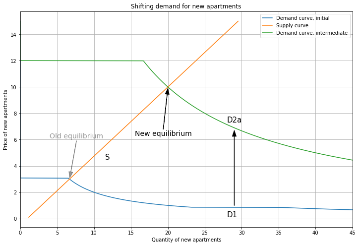
Next, the rich Person 3 moves in. This shifts the demand curve for new apartments up (from D1 to D2a), resulting in a new equilibrium at \(P_{New} = 10\). But now supply intersects demand on the segment where only Person 3 buys, so Person 2 has been priced out and will downgrade to an Old apartment.

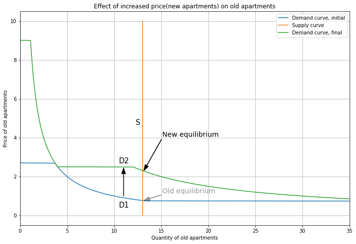
The increased price of New apartments makes Old apartments more attractive, so demand for Old apartments shifts up. Now supply intersects demand on the segment where both Person 1 and Person 2 buy, and the price rises from 0.8 to 2.3. The stock of 13 Old units is now shared by both Person 1 and 2. This is the demand cascade: rich people moving in and increasing competition in the market for new apartments results in higher prices of old apartments, making housing less affordable for the poor. (This is also known as up-filtering, where for a given home, poorer residents are replaced by richer residents.) Here I’ve shown how demand cascades over two steps; in reality, demand would flow down dozens of steps, representing different levels of housing quality.

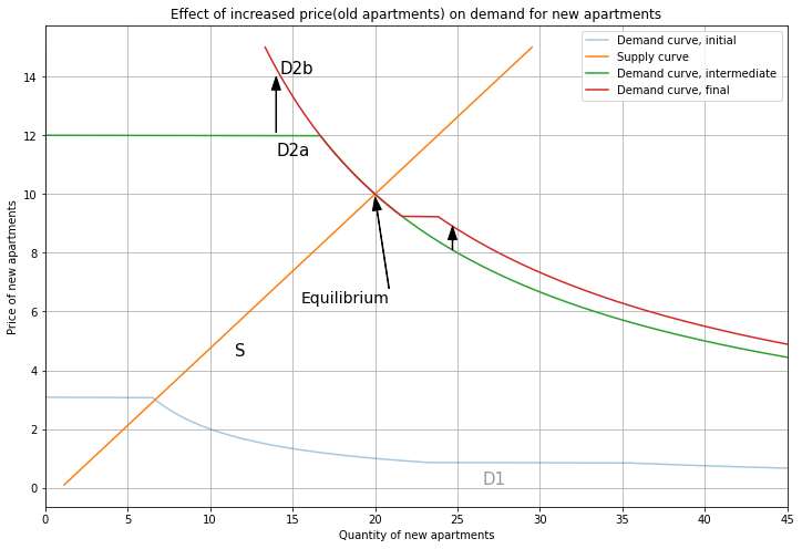
To finish up the new equilibrium, we account for the effect of the higher price(Old) on the New market. Higher prices for Old apartments make New apartments for attractive, so demand shifts up (from D2a to D2b), but this doesn’t change the equilibrium.

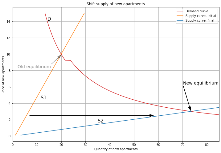
Now let’s use a yuppie fishtank to reverse the effects of the demand cascade. We’ll increase the supply of new apartments enough to offset the increased demand from Person 3. Supply shifts from S1 to S2, and the price falls from 10 back to 3. Now supply intersects demand on the segment where both Person 2 and 3 buy, so Person 2 has upgraded from Old to New (just as in the vacancy chain).

Since Person 2 upgrades, demand for Old apartments goes back to the original level, and the price falls to 0.8. This is the yuppie fishtank: by building new apartments, we absorb the demand of rich newcomers and prevent prices of old housing from rising.

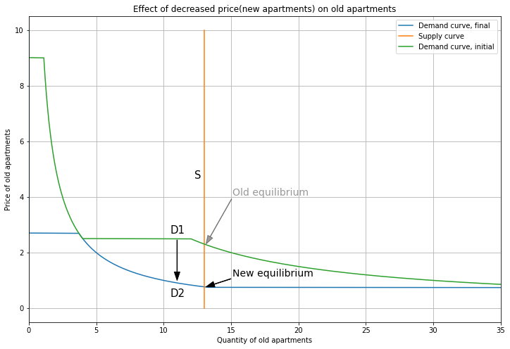
Tidying up, the fall in price(Old) shifts demand for New apartments down, but the equilibrium is unchanged.

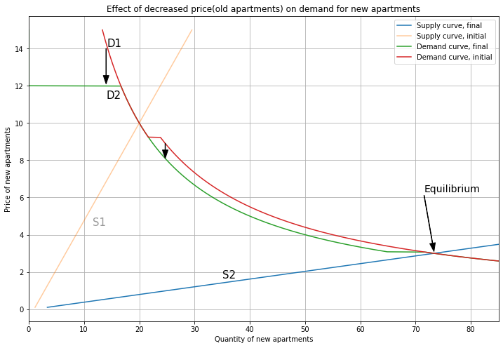
To conclude, note that vacancy chains and yuppie fishtanks are closely related. A vacancy chain allows a local resident to upgrade, reducing demand for old housing. A yuppie fishtank absorbs demand from a rich newcomer, preventing a demand increase for old housing. And the reversal tests work as expected. Reducing the supply of new apartments (say, a new building burns down) causes a demand cascade, while reducing demand for new apartments (say, deporting yuppies) creates a vacancy chain.

---

See here and here for code to produce the graphs.