Did medical marijuana legalization reduce crime? A replication exercise
Summary
In this post I replicate the paper “Is Legal Pot Crippling Mexican Drug Trafficking Organisations? The Effect of Medical Marijuana Laws on US Crime” by Gavrilova, Kamada, and Zoutman (Economic Journal, 2019; replication files).
I find three main problems in the paper:
- it uses weighting when its own justification doesn’t apply
- it uses a level dependent variable, and isn’t robust to log-level or Poisson models
- it does not test for pretrends in the disaggregated crime variables, and two alternative event studies show that the results are driven by differential trends
Introduction
This paper studies the effect of medical marijuana legalization on crime in the U.S., finding that legalization decreases crime in states that border Mexico. The paper uses a triple-diff method, essentially doing a diff-in-diff for the effect of legalization on crime, then adding an interaction for being a border state.
The paper uses county level data over 1994-2012, with treatment (medical marijuana legalization, MML) occurring at the state level. The authors use “violent crimes” as the outcome variable in their main analysis, defined as the sum of homicides, robberies, and assaults, where each is measured as a rate per 100,000 population. They also perform separate analyses for each of the three crime categories.
The basic triple-diff regression is:
\[y_{cst} = \beta^{border} D_{st}B_{s} + \beta^{inland} D_{st} (1-B_{s}) + \gamma_{c} + \gamma_{t} + \varepsilon_{cst}.\]Here \(y_{cst}\) is the outcome in county \(c\) in state \(s\) in year \(t\); \(D_{st}\) is an indicator for having enacted MML by year \(t\); \(B_{s}\) is an indicator for bordering Mexico; \(\gamma_{c}\) are county fixed effects; \(\gamma_{t}\) are year fixed effects. The full model also includes time-varying controls, border-year fixed effects, and state-specific linear time trends. The outcome is crime rates per 100,000 population, measured in levels, so the regression coefficients will not have a percentage interpretation; we’ll come back to this later.
This isn’t a standard triple-diff. In this model, \(\beta^{border}\) is capturing the absolute effect of MML in border states, and not the differential effect relative to inland states. To see this, compare to:
\[y_{cst} = \beta^{DD} D_{st} + \beta^{DDD} D_{st} \times B_{s} + \gamma_{c} + \gamma_{t} + \varepsilon_{cst}.\]Here, \(\beta^{DD}\) represents the effect of MML in inland states, and \(\beta^{DDD}\) is the differential effect in border states (relative to the effect in inland states). That is, \(\beta^{inland} = \beta^{DD}\) and \(\beta^{border} = \beta^{DD} + \beta^{DDD}\). This is perhaps an issue of taste. What I would primarily want to know is whether MML had a larger effect in border states relative to inland states; the absolute effect in border states is secondary. Hence, I will report results from the second model (although the differences are small, because the inland effect is small: \(\beta^{inland} = \beta^{DD} \sim 0\)).
The authors find that, on average, MML reduces violent crimes by 35 crimes per 100,000 population, but the estimate is not statistically significant (the standard error is 22). Then, zooming in on the border states, they find a significant reduction of 108 crimes per 100,000 (and a nonsignificant increase of 2.8 in inland states). There are three border states that legalized medical marijuana: California, New Mexico, and Arizona. (Texas is the remaining border state.) Splitting up the effect by treated border state, we have a reduction of 34 in Arizona, 144 in California, and 58 in New Mexico.
I don’t really like this “zoom in on the significance” style of research. We can always find significance if we run enough interactions. And as we zoom in on subgroups, we lose external validity: can we make meaningful predictions for a state or country that was legalizing marijuana and didn’t border on Mexico? Moreover, the identifying assumptions become harder to believe. When n=3, it’s more plausible that differential shocks are driving the result (compared to n=20, say). That is, it could be that crime was already decreasing in the three border states when they passed MML, and the negative correlation between MML and crime is coincidental.
Ok, let’s get into the issues.
Weighting
The authors use weighted least squares (weighting by population) for their main results. They justify weighting by performing a Breusch-Pagan test, and finding a positive correlation between the squared residuals and inverse population. This implies larger residuals in smaller counties. In other words, there is heteroskedasticity, and weighting will decrease the size of the standard errors, i.e., increase precision. However, in Appendix Table D7, you’ll note that while they get a positive correlation when using homicides and assaults as the dependent variable, this coefficient is negative and nonsignificant for robberies. So by the Breusch-Pagan test, the robbery results actually should not be weighted. And in Table D9, the unweighted robbery estimate has smaller standard errors than the weighted one: weighting is reducing precision. And yet, the paper still uses weighting when estimating the effect of MML on robberies (in Table 4). We’ll see below that this makes a big difference for the effect size.
Modelling the dependent variable
The authors estimate the effect of MML on crime using a level dependent variable instead of taking the logarithm, which I had thought was standard. In particular, their main results use the aggregate crime rate, which leads to a “level” interpretation: MML reduces the crime rate by \(\hat{\beta}=\) 108 crimes per 100,000 population.
I would have used a log-level regression, taking \(log(y+1)\) for the dependent variable (adding 1 if there are zeroes in the data), which gives a percentage (or semi-elasticity) interpretation: MML reduces crime by \(100 \times (exp(\hat{\beta})-1) \%\). The paper doesn’t justify why they don’t use a log-level model. This is even more surprising when you see that they manually calculate the semi-elasticity (p.19), again without mentioning the log-level approach.
After spending some time looking into this question of logging the dependent variable for skewed, nonnegative data, I’m still pretty confused. It seems the options are: (1) level-level regression, as used in this paper; (2) log-level regression; (3) transforming \(y\) with the inverse hyperbolic sine; and (4) Poisson regression (with robust standard errors, you don’t need to assume mean=variance). But it’s not clear what the “correct” approach is. I’d expect a true result to be robust across multiple approaches, so let’s try that here.
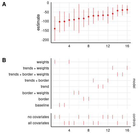
I estimate the triple-diff model using a level-level regression (to directly replicate the paper), a log-level regression, and a Poisson regression. (The inverse hyperbolic sine approach is almost identical to log-level, so I skip it here.) To see how the specification matters, I conduct a specification curve analysis using R’s specr package. Specifically, I run all possible combinations of model elements, either including or excluding covariates, population weights, state-specific linear time trends, and border-year fixed effects. This will allow us to see whether possibly debatable modelling choices, such as state-specific linear trends, are driving the results.
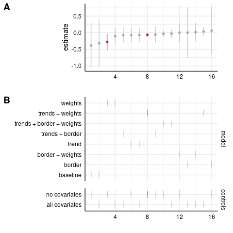
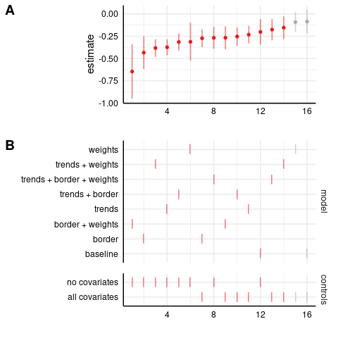
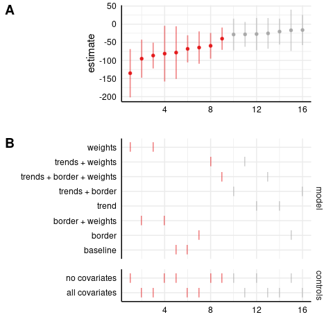
Here are the homicide results, first in the level-level model (as in the paper). Panel A plots the coefficient estimates in increasing order, while panel B shows the corresponding specification. Each specification has two markers in panel B, one in the upper part indicating the model, and one in the lower part indicating whether all or no covariates are included in the model.1 For example, the specification with the most negative estimate is ‘trends + weights, no covariates’. In both panels, the x-axis is just counting the number of specifications, and the color scheme is: (red, negative and significant), (grey, insignificant), (blue, positive and significant). The ‘baseline’ specification omits the state-specific trends, border-year fixed effects, and doesn’t weight by population. I’ll be focusing on the full specification, ‘trends + border + weights, all covariates’, which includes state-specific linear trends, border-year fixed effects, and weights by population.
Level-level model: homicides
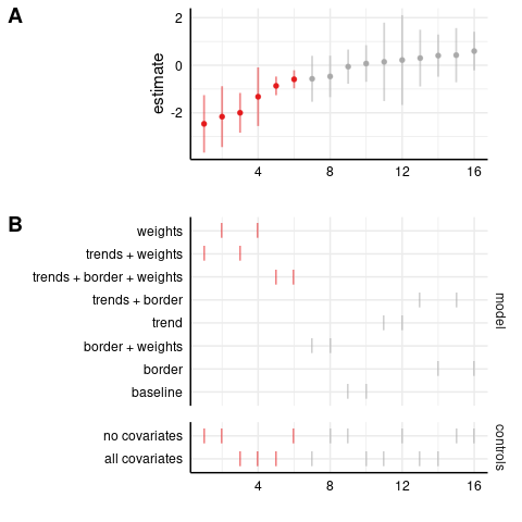 We can see that the estimate is negative and statistically significant in the full specification, with and without covariates.
Most estimates are nonsignificant; these are generally the unweighted models, indicating the importance of population weighting for these results.
We can see that the estimate is negative and statistically significant in the full specification, with and without covariates.
Most estimates are nonsignificant; these are generally the unweighted models, indicating the importance of population weighting for these results.
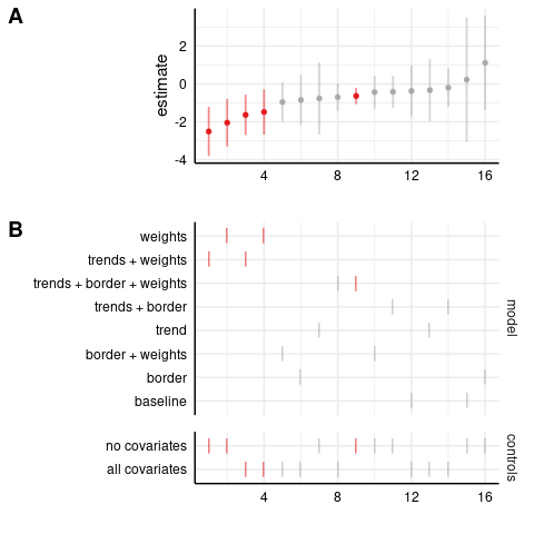
Log-level model: homicides
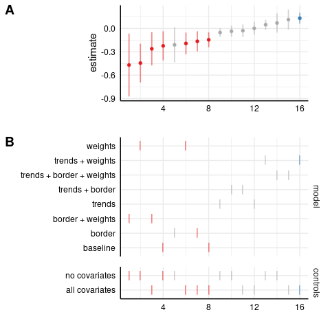
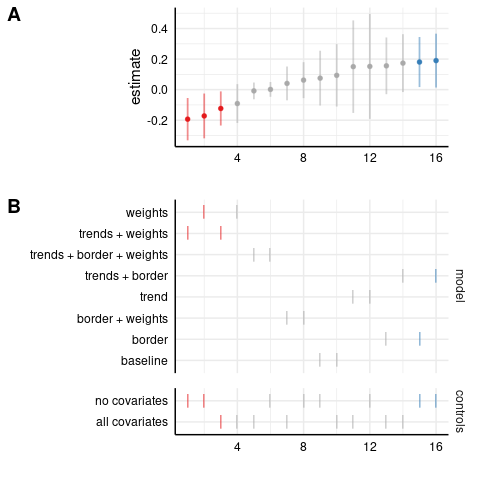 Next, in the log-level model, most estimates are insignificant, including the full specification.
Two models even have positive and significant results (in blue). Let’s see the Poisson model:
Next, in the log-level model, most estimates are insignificant, including the full specification.
Two models even have positive and significant results (in blue). Let’s see the Poisson model:
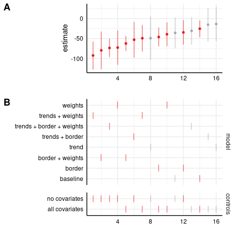
Poisson model: homicides
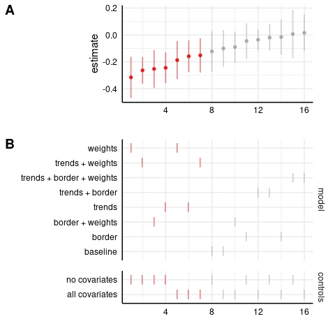 Here I use the homicide count (instead of the rate per 100,000 population), though note that the controls include log population and I’m weighting by population.
In this case, the estimates are almost exactly zero and nonsignificant in the full specification.
So, the homicide results only go through using the level-level regression, and not in the log-level or Poisson models.
Here I use the homicide count (instead of the rate per 100,000 population), though note that the controls include log population and I’m weighting by population.
In this case, the estimates are almost exactly zero and nonsignificant in the full specification.
So, the homicide results only go through using the level-level regression, and not in the log-level or Poisson models.
For the other dependent variables, I’ll show the graphs in the footnotes. The results for robberies are more robust. The full specification is negative and significant across all three models.2 However, the assault results are not robust, with the full specification nonsignificant for both log-level and Poisson regressions.3
This doesn’t look great for the paper. I’d expect real effects to be robust across the three models. I conclude that at best, the paper provides evidence for an effect of MML on robberies in border states, but not on homicides or assaults. And this is assuming the event study graph looks good for pretrends, which I’ll discuss next.
Event study
There are big trends in crime over this period. Crime fell a lot during the 90s, and again after 2007. To show that their results aren’t driven by these trends, the authors present an event study graph in Figure 6, estimating a triple-diff coefficient in each year. Basically, this is estimating the triple diff for each year relative to an omitted period.
The authors estimate their main results using the 1994-2012 sample. For the event study, they also use an extended sample from 1990-2012. The extended sample has issues, because it uses flawed imputed data over 1990-1992, and the year 1993 is missing entirely. Here I will show results from the main sample, 1994-2012.
For their main event study, the authors only include dummies for relative years -2 to 4, and bin all years 5+ in one dummy. This is because California is treated in 1996 and only has two years of pretreatment data, and wouldn’t contribute to any dummies before -2.4 But this is a bit of an arbitrary choice. Similarly, Arizona is treated in 2010 and only has two years of post-treatment data, and hence doesn’t contribute to any dummies after +2. So should we include dummies only for [-2,2]?
I think it’s fine to include dummies for [-5,5], with the understanding that some states do not contribute to some estimates. (Specifically, California doesn’t have dummies for -5 to -3, and Arizona doesn’t have dummies for 3 to 5+.) In this setup, the omitted years are <-5, in contrast to the standard approach of omitting relative year -1. (As noted in the last footnote, California has no omitted years, so the software should drop one year.)
Next I plot my version of their event study graph, using a level dependent variable. Since this is a triple-diff, I include relative year dummies for the treated states, as well as separate relative year dummies for the treated border states. I plot the coefficients on the border-state relative year dummies. While the paper only includes dummies for [-2,5+], I estimate coefficients for [-5,5+].5
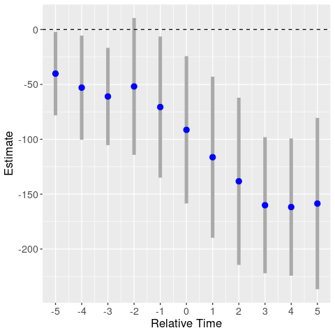
Event study: violent crimes (binning 5+)
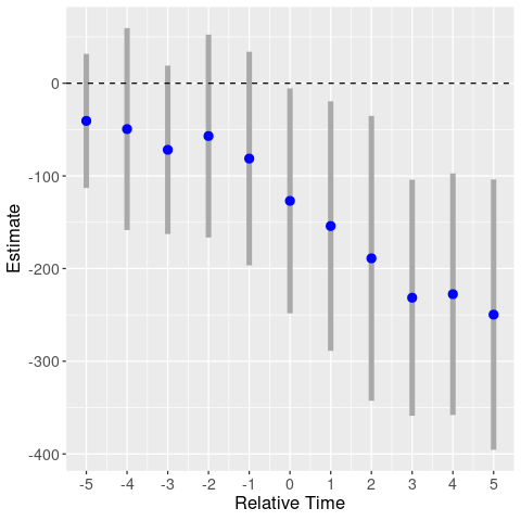
Compared to the event study in the paper, here the coefficients are all negative. For the pretreatment estimates (treatment occurs in period 0), this means level differences between the treated border and inland states. There is also a slight downward trend before the treatment, hinting at differential trends.
In any case, note that this graph is for the aggregated violent crime variable. Where are the event studies for the individual dependent variables? The authors do not show them! This is a major flaw, and I can’t believe that the referees missed it. Even if we found no pretrends in the aggregate variable, there could still be pretrends in the component variables. Let’s take a look ourselves.
Event study: homicides (binning 5+)
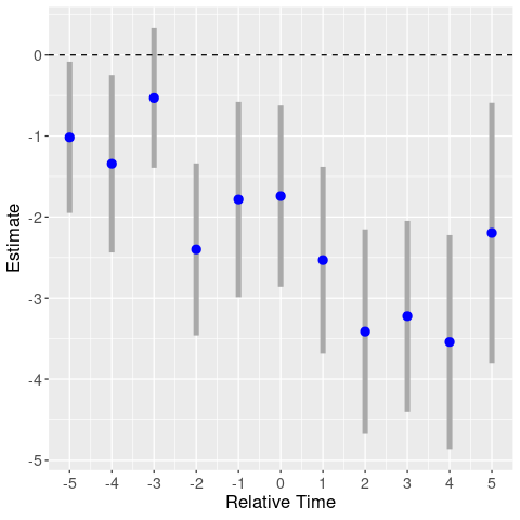 First up, using the homicide rate as the dependent variable, we get a big mess.
There are big movements in years -3 and -2: relative to the treatment year, homicides were higher three years prior, and lower two years prior.
So at least for homicides, it looks like the negative triple-diff estimate could just be picking up noise.
Now we know why the authors didn’t include separate event study graphs by dependent variable.
First up, using the homicide rate as the dependent variable, we get a big mess.
There are big movements in years -3 and -2: relative to the treatment year, homicides were higher three years prior, and lower two years prior.
So at least for homicides, it looks like the negative triple-diff estimate could just be picking up noise.
Now we know why the authors didn’t include separate event study graphs by dependent variable.
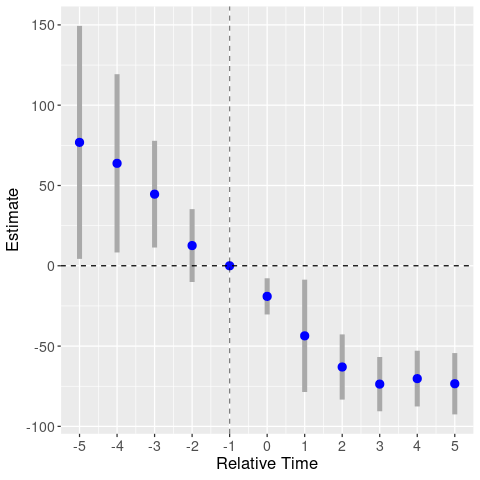
Event study: robberies, unweighted (binning 5+)
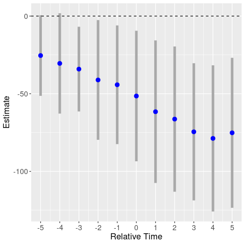 For robberies, recall that the Breusch-Pagan test failed to justify weighting, so I do not use weights.
Here, it also looks like a negative trend is driving the result: robberies were smoothly decreasing in treated border states before MML was implemented. (See the unweighted graph in the footnote.6)
The common trends assumption for the triple-diff appears to be violated.
For robberies, recall that the Breusch-Pagan test failed to justify weighting, so I do not use weights.
Here, it also looks like a negative trend is driving the result: robberies were smoothly decreasing in treated border states before MML was implemented. (See the unweighted graph in the footnote.6)
The common trends assumption for the triple-diff appears to be violated.
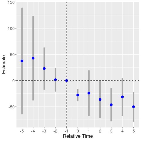
Event study: assaults (binning 5+)
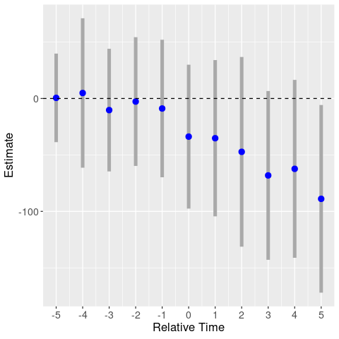 Finally, for assaults, the event study actually doesn’t look bad, although the standard errors are large.
This is a bit surprising, given that the assault results were not robust across log-level and Poisson models.
Finally, for assaults, the event study actually doesn’t look bad, although the standard errors are large.
This is a bit surprising, given that the assault results were not robust across log-level and Poisson models.
Overall, this doesn’t look good for the paper. I think this is an equally defensible event study method, but it nukes their homicide and robbery results.7
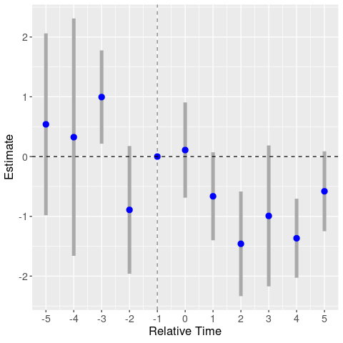
I’m not a fan of binning in event studies. In Andrew Baker’s simulations, binning periods 5- and 5+ performs badly. In contrast, a fully-saturated model including all relative year dummies (except for relative year -1, which is the omitted year) performs perfectly. So let’s try that here.
By omitting year -1, we’re basically normalizing the above event study graphs around the -1 estimate (but also changing the estimates, since we’re including all other relative year dummies). Hence, the homicide graph has the same patterns, but shifted up. We again find a clear trend in the robbery graph. But now the assault graph also looks to be driven by trends.
Event study: homicides
Event study: robberies
Event study: assaults
Takeaway: now I really doubt that MML had a causal effect on crime.
Synthetic control
To further dig into these trends, I aggregated the data from county- to state-level and performed a synthetic control analysis for each of the three treated border states: California, Arizona, and New Mexico. This aggregation is probably imperfect, and it would be better to start with state-level data, but let’s see what happens. (Running level-level regressions, I still get negative results, with effect sizes similar to the county-level data. See the specification curves in the footnote. 8)
The idea of synthetic control is to construct an artificial control group for our treated state, so we can evaluate the treatment effect simply by comparing the outcome variable in the treatment and synthetic control states. The synthetic control group is a weighted average of control states, and these weights are chosen to match the treated state on preperiod trends. I use the nevertreated states as the donor pool; I’ll report the weights below.
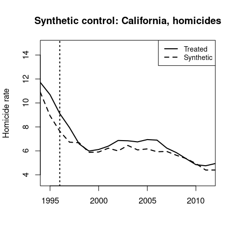
Here I’ll show the robbery results for the three states (using the level dependent variable), to see what’s happening with that smooth trend. Note that these graphs are plotting the raw outcome variable, so we’re seeing the actual trends in the data.
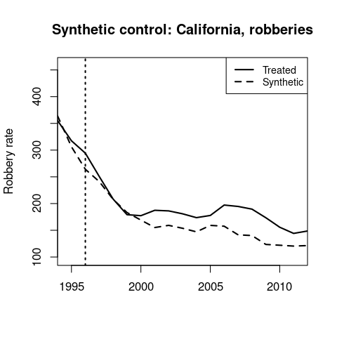 California’s synthetic control is 68% New York and 28% Minnesota.
California’s MML occurs in the middle of the 1990s crime decrease, and it doesn’t look like there’s much of an effect in 1996.
California’s synthetic control is 68% New York and 28% Minnesota.
California’s MML occurs in the middle of the 1990s crime decrease, and it doesn’t look like there’s much of an effect in 1996.
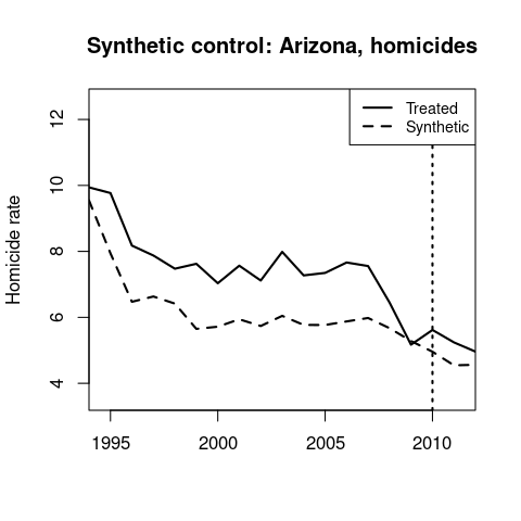
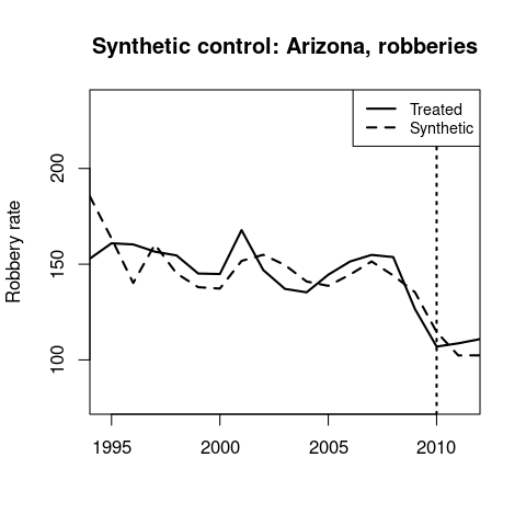 Arizona’s synthetic control is 61% Texas, 24% Florida, and 15% Wyoming.
Again, there doesn’t seem to be a treatment effect.
Arizona’s synthetic control is 61% Texas, 24% Florida, and 15% Wyoming.
Again, there doesn’t seem to be a treatment effect.
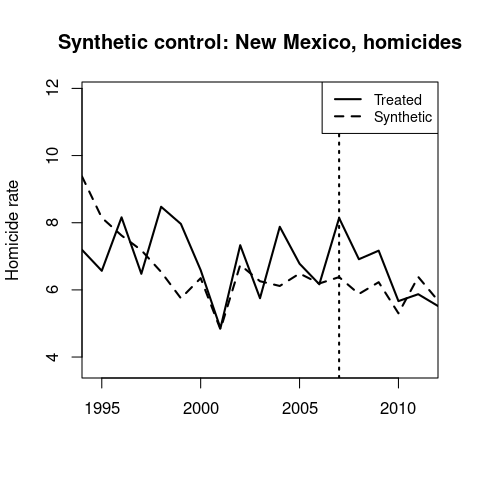
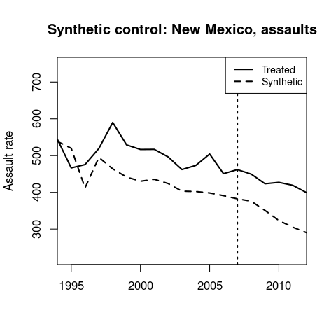
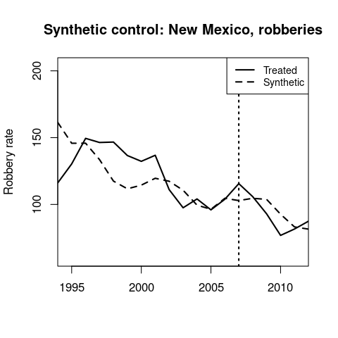 New Mexico’s synthetic control is 51% Mississippi, 21% Louisiana, 18% Texas, and 7% Wyoming.
Its MML occurs before a drop in robberies that is partly matched by the synthetic control group.
New Mexico’s synthetic control is 51% Mississippi, 21% Louisiana, 18% Texas, and 7% Wyoming.
Its MML occurs before a drop in robberies that is partly matched by the synthetic control group.
You can look at the other synthetic control graphs in this footnote.9
Overall, I worry that these three states coincidentally legalized medical marijuana when crime was high and falling, and that the triple-diff estimates are just picking up these trends. Based on my analysis here, I don’t believe that medical marijuana legalization reduced crime in the US.
Randomization inference
One final note: the paper calculates a (one-sided) randomization inference p-value of 0.03, and claims that this is evidence for their result being real. However, as I discuss in this post, this claim is false. With large sample sizes, there’s no reason to expect RI and standard p-values to differ, so a significant RI p-value provides no additional evidence.
Conclusion
I think it’s plausible that moving marijuana production from the black market to the legal market would reduce crime (at least in the long run). But the effect of medical marijuana legalization on crime is too small to detect in the data.
Footnotes
See here for R code, and here for the original replication files. (For some reason, the replication files aren’t online anymore.)
PS: Table 5 does heterogeneity by type of homicide; I’d be curious to see the event study for each of these outcomes.
-
The full covariate list is: an indicator for decriminalization, log median income, log population, poverty rate, unemployment rate, and the fraction of males, African Americans, Hispanics, ages 10-19, and ages 20-24. In general, I find that adding controls barely changes the \(R^{2}\), so these variables aren’t adding much beyond the county and year fixed effects. ↩
-
Robbery results:
Level-level model: robberies
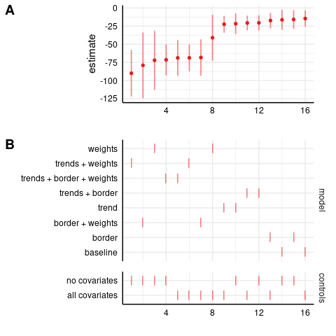 In the level-level model, we see a big difference between the weighted and unweighted results. Clearly, there are heterogeneous treatment effects, with larger effects in the higher-weight states (California, probably).
As I noted above, the robbery estimates should not be weighted.
In the level-level model, we see a big difference between the weighted and unweighted results. Clearly, there are heterogeneous treatment effects, with larger effects in the higher-weight states (California, probably).
As I noted above, the robbery estimates should not be weighted.Log-level model: robberies
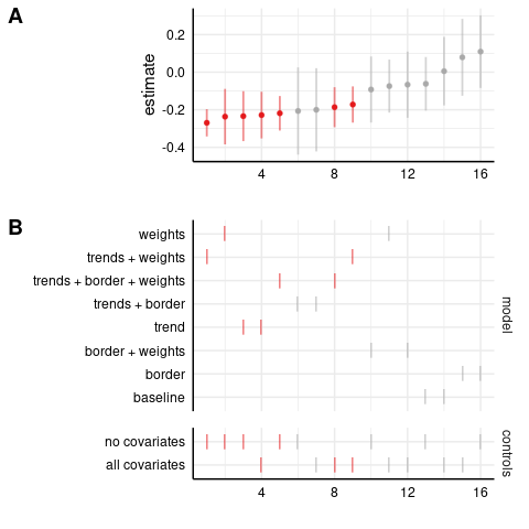
Poisson model: robberies
-
Assault results:
Level-level model: assaults
Log-level model: assaults
Poisson model: assaults
-
One problem with this specification is that California has no omitted years. Every year from 1994-2012 has a dummy variable, which seems like a dummy variable trap (i.e., multicollinearity). Specifically: 1994-2000 are covered by dummies for -2 to 4, and 2001-2012 are covered by the 5+ binned dummy. ↩
-
Moreover, as noted above, I am estimating the differential effect of MML in border states relative to inland states, while GKZ are estimating the absolute effect. I also drop counties that have the black share of population greater than 100%. It seems the authors were doing some extrapolation that got out of control. ↩
-
We shouldn’t care about this graph, because weighting is unwarranted.
Event study: robberies, weighted (binning 5+)
-
It’s depressing that event studies can differ so much based on slight model changes. I have a feeling that a lot of diff-in-diffs from the past twenty years are not going to survive replication. ↩
-
Specification curve for state-level results:
Level-level model: homicides
Level-level model: robberies
Level-level model: assaults
-
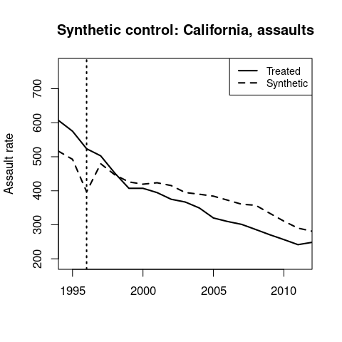
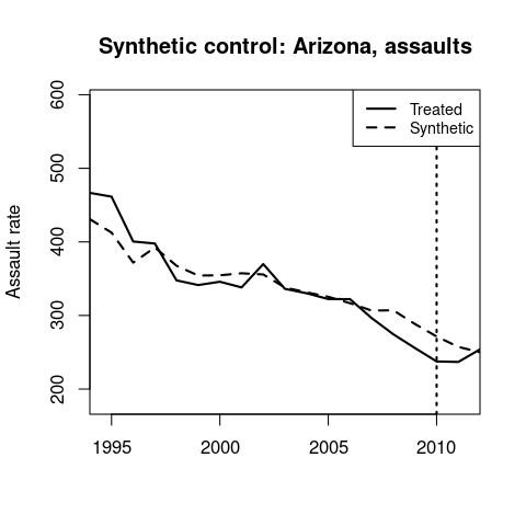
Synthetic control results for homicides and assaults.
 ↩
↩
 Michael Wiebe
— built with Jekyll using Lagom theme
Michael Wiebe
— built with Jekyll using Lagom theme