Introduction

Moretti (2021) (original code, my code, code walkthrough video) studies agglomeration effects for innovation, testing whether the size of technology clusters causes patenting. Agglomeration effects are important for understanding technological progress (Kerr and Robert-Nicoud, 2020), and are affected by constraints on housing supply (Hsieh and Moretti, 2019, Duranton and Puga, 2020). Using US data on patents filed between 1971 and 2007, Moretti presents multiple lines of evidence supporting a causal effect of cluster size on patenting. The main results are from OLS regressions of patents on cluster size, controlling for an extensive set of fixed effects. Moretti addresses identification concerns using an event study and an instrumental variables strategy. The event study, using inventors who change cities, tests for selection bias from promising inventors sorting into large clusters. The instrument uses variation in the number of inventors in other cities to control for omitted variable bias from sources like local field-specific subsidies.

In this comment, I identify coding errors that overturn the results from the event study and the instrumental variables regressions. First, the event study does not interact the treatment variable with a time indicator in the year of the treatment. Including the correct interaction produces a nonsignificant effect in \(t=0\). Second, the instrument is constructed by incorrectly taking first-differences across cities, due to not sorting the data by city. When I calculate the first-difference within cities, the first stage and 2SLS estimates are both nonsignificant. Hence, the positive correlations from the OLS regressions could be biased upwards due to sorting and omitted variable bias.

Event study

In Figure 6, Moretti uses an event study to address worries about sorting, where ‘rising star’ inventors (with increasing patent counts) in small clusters are systematically hired by employers in large clusters.¹ If these promising inventors select into larger clusters, then the positive correlation between cluster size and patenting need not represent a causal effect of cluster size. Note that the main results control for inventor fixed effects, so the threat to identification comes only from inventors whose inventiveness is increasing over time. If sorting does occur, we should observe patenting rising in the years before an inventor moves to a new city.

To test for sorting, Moretti performs an event study using variation in cluster size from inventors who move across cities exactly once. That is, ‘stayers’ who never move are excluded, so the event study does not have a never-treated group. To generate a treatment-control comparison, Moretti uses average cluster size before and after the move as a continuous treatment variable. Specifically, Moretti interacts pre-move average cluster size with the pre-move event-time indicators, and post-move average cluster size with the post-move event-time indicators.² The implied regression equation is \(\begin{aligned} \begin{split} \label{eq:es} \text{ln} y_{ijfct} &= \sum_{s=-5}^{-1} \beta_{s} \text{Size}^{pre}_{-ifc} \times 1\{t=s\} + \sum_{s=0}^{5} \beta_{s} \text{Size}^{post}_{-ifc} \times 1\{t=s\} \\ &+ d_{cf} + d_{ck} + d_{ft} + d_{kt} + d_{ct} + d_{i} + d_{j} + \varepsilon_{ijfkct}. \end{split}\end{aligned}\)

Here \(y\) is the number of patents by inventor \(i\) in firm \(j\), research field \(f\), city \(c\), and year \(t\); \(k\) is the research class.

The event study results are driven entirely by one coding error. Moretti did not generate an interaction of post-move cluster size with a \(t=0\) indicator, but instead uses the time-varying cluster size variable used in the OLS regressions. Hence, \(\beta_{0}\) is estimated using data from all event-years, instead of capturing the effect in \(t=0\). I correct the code by interacting post-move cluster size with the \(t=0\) indicator.³ Below I’ve included a snippet of the original code with the error.

* cluster size and number of patents
gen x = log(Den_bea_zd)
gen y = log(number)

* event time
gen tt = year - move_year1

* average cluster size before and after the move
egen tmp_mm = mean(x) if tt >= -5 & tt <=-1, by(inventor)
egen tmp_pp = mean(x) if tt >= 1  & tt <= 5, by(inventor)
egen tmp_m = max(tmp_mm),  by(inventor)
egen tmp_p = max(tmp_pp),  by(inventor)

* year indicators
g m1 = (tt==-1)
g m2 = (tt==-2)
g m3 = (tt==-3)
g m4 = (tt==-4)
g m5 = (tt==-5)
g p1 = (tt==1)
g p2 = (tt==2)
g p3 = (tt==3)
g p4 = (tt==4)
g p5 = (tt==5)

* interact treatment variables with year indicators
g x_m1 = tmp_m*m1
g x_m2 = tmp_m*m2
g x_m3 = tmp_m*m3
g x_m4 = tmp_m*m4
g x_m5 = tmp_m*m5
g x_p1 = tmp_p*p1
g x_p2 = tmp_p*p2
g x_p3 = tmp_p*p3
g x_p4 = tmp_p*p4
g x_p5 = tmp_p*p5

* note that B_0 is estimated using `x`, defined above as time-varying cluster size:
reghdfe y x_p5 x_p4 x_p3 x_p2 x_p1 x x_m1 x_m2 x_m3 x_m4 x_m5, absorb(year bea zd class cluster1 cluster_bea_class cluster_zd_year cluster_class_year inventor cluster_bea_year org_new) vce(cluster cluster1)

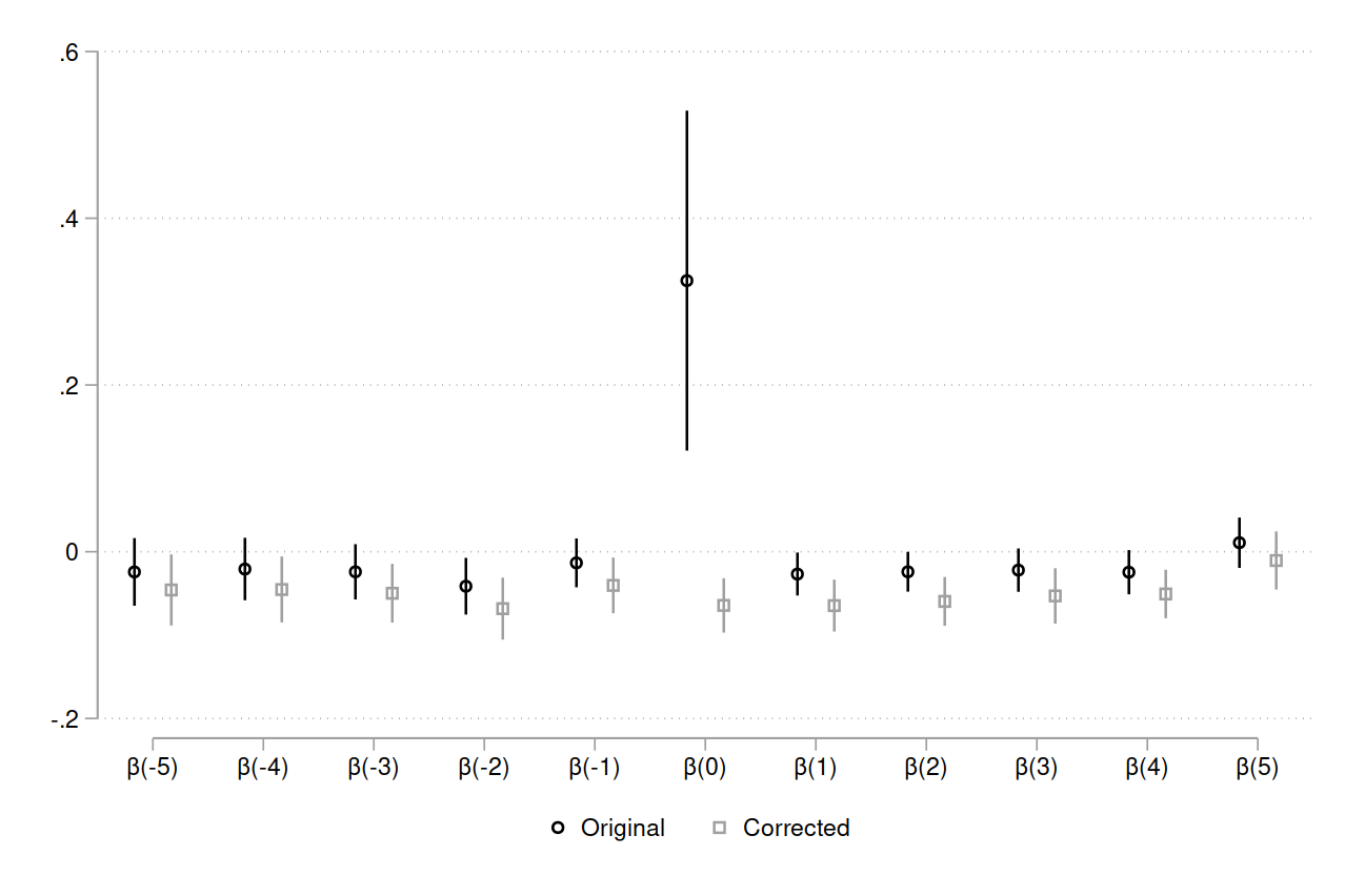
Figure 1: Replication and correction of Figure 6 event study Note: Event study coefficients from Equation 1. Original estimates \(\beta_{0}\) using time-varying Size\(_{-ifct}\) and without interacting with \(1\{t=0\}\). Corrected estimates \(\beta_{0}\) using Size\(^{post}_{-ifc} \times 1\{t=0\}\); following Moretti, Size\(^{post}_{-ifc}\) is calculated excluding \(t=0\). N=18,433 in Original, N=18,434 in Corrected. Standard errors are clustered by city \(\times\) research field. Moretti’s Figure 6 switches the leads and lags, for example, putting \(\beta_{-5}\) as the last coefficient and \(\beta_{5}\) as the first.

Figure 1 shows the original and corrected event studies.⁴ The large effect in \(t=0\) disappears when using the correct specification. Hence, Moretti does not provide evidence against bias in the OLS results from sorting, where promising inventors select into large clusters. Moreover, if agglomeration effects are real, we should detect them using a mover event study. So the absence of an effect in the corrected event study should lead us to discount the main findings.⁵ However, since there are 118,000 inventors in the OLS sample and only 3,000 in the event study sample, the size of this discount should be small. Finally, since inventors move in different years, note that this is a staggered adoption design where a two-way fixed-effects estimator may be biased.⁶

Instrumental variables estimates

In Table 5, Moretti uses an instrumental variables strategy to address worries about omitted variable bias, where cluster size is correlated with unobserved time-varying shocks at the city-field level. For example, a city subsidizing biotech firms could increase both biotech patents and the size of the biotech cluster.⁷ The idea for the instrument is to use variation in the number of inventors in other cities who are employed by firms that are also active in the focal inventor’s city.

To illustrate with an example, for the focal inventor \(i\) in the field of computer science at Google in San Francisco, we instrument for cluster size using variation in the number of computer science inventors at Microsoft in Seattle, where Microsoft also has inventors in San Francisco. Intuitively, the number of inventors working at Microsoft in Seattle will be correlated with the number of computer science inventors in San Francisco, since Microsoft also has a presence in San Francisco, allowing shocks to Microsoft to propagate to San Francisco. The exclusion restriction is that, controlling for fixed effects, the number of computer science inventors at Microsoft in Seattle is not directly correlated with computer science patents at Google in San Francisco. While this example uses two firms, the instrument uses all firms active in the focal inventor’s city, excluding the inventor’s own firm.

In contrast to the OLS results, Moretti defines the instrument in first-differences. Let \(\Delta N_{jf(-c)t} = N_{jf(-c)t} - N_{jf(-c)(t-1)}\) be the first-difference over time in the number of inventors at firm \(j\) in research field \(f\) in all cities excluding \(c\), and let \(\Delta N_{ft}\) be the national change by field. With \(D_{jfc(t-1)}\) as an indicator for firm \(j\) employing at least one inventor in city \(c\) and field \(f\) in year \(t-1\) (so that the first-difference is well-defined), the IV is

where the sum is taken across all firms excluding \(j\).

The regression equation is

where \(y\) is the number of patents, \(S\) is cluster size (excluding the focal inventor \(i\)), and \(k\) is research class.

There are two coding errors that affect the IV results. First, when calculating the first-differenced term \(\Delta N_{jf(-c)t}\), Moretti sorts the data by firm, field, and year, but not by city. This means that the first-difference is taken across different cities, instead of within the focal city. Hence, the code generates an incorrect instrument that does not match the definition in the text. I correct the code to sort by city and take first-differences within city. See the code snippet below.

* number of inventors by firm-year-field-city
egen r2 = sum(n), by(org_new year zd bea)

* number of inventors by firm-year-field
egen rr2 = sum(n), by(org_new year zd)

* number of inventors outside of the focal city
g DD = rr2 - r2

* first-difference
* note: not sorting by city (bea)
sort zd org_new year
by zd org_new: g DD1 = DD - DD[_n-1]

Moreover, the code generates unreproducible results. This is because firm-field-year is not a unique sorting order, as there are observations with the same values for firm-field-year but in different cities. Since Stata’s sort command randomly orders the data before sorting, each run of the code results in a different sorting by city within tied values of firm-field-year. Hence, the first-difference is calculated differently each time. In Figure 2, I show the variance in the original results from 500 iterations of generating the instrument and running the same regression.

Figure 2: Distribution of coefficients and t-statistics from 2SLS regression 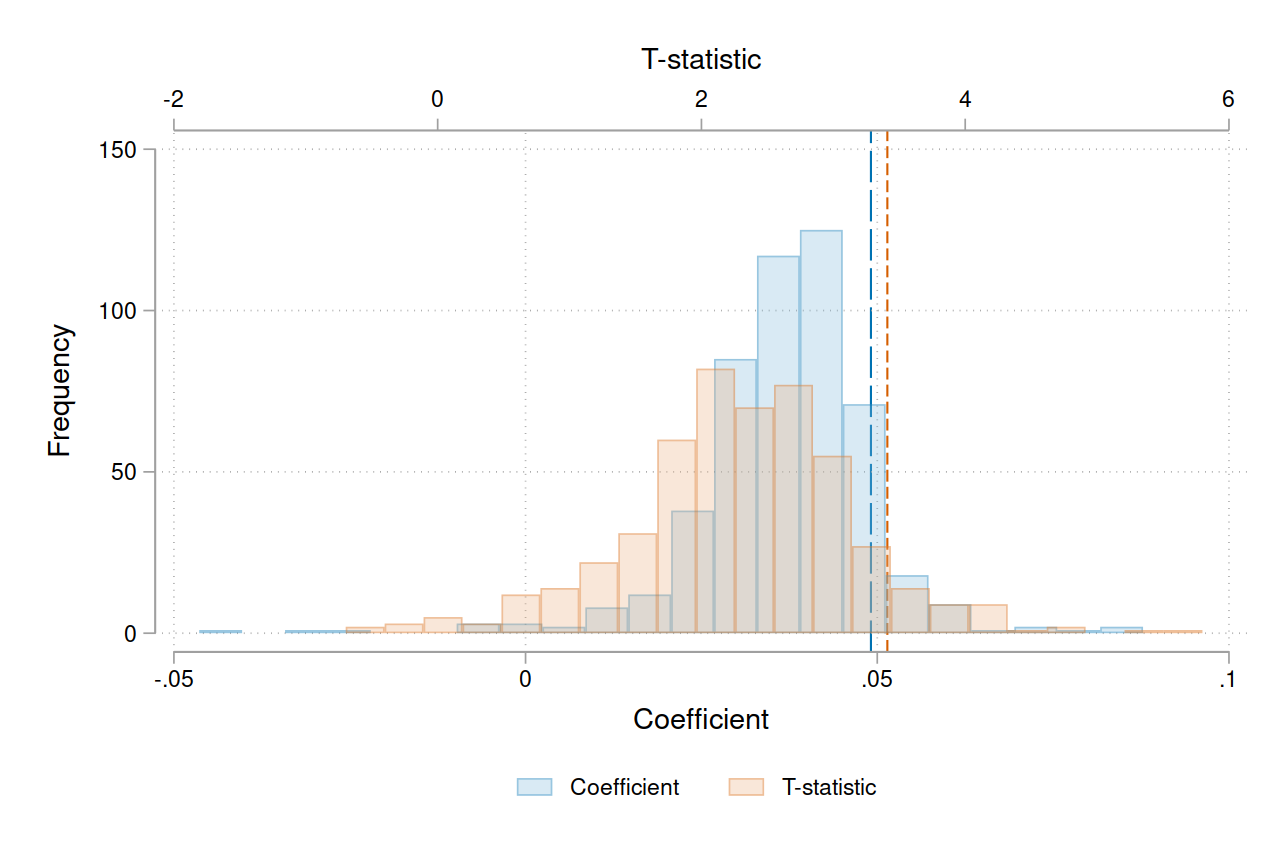Note: Estimation results from the 2SLS regression in Table 5, Column 6. The distribution is constructed from 500 iterations of generating the instrument and running the regression. The original code sorts by firm-field-year but not city, which leads to a random ordering by city within tied values of firm-field-year. The first-difference in the numerator of the instrument is then (incorrectly) taken across cities, which causes the instrument to be different for each run of the code. The original estimate is 0.0491 (blue long-dashed line) with a t-statistic of 3.41 (orange short-dashed line).

The second error is that Moretti’s code incorrectly defines the instrument for all observations, including observations for which \(\Delta N_{sf(-c)t}\) is missing (because the first-difference is taken across firms, cities, or non-consecutive years). Specifically, Moretti calculates \(\sum_{s \neq j} D_{sfc(t-1)} \frac{\Delta N_{sf(-c)t}}{\Delta N_{ft}}\) by first calculating the sum over all firms (by field-city-year), and then subtracting the value for the focal firm \(j\). However, the code assigns the field-city-year total to all firms, and subtracts the summand for firm \(j\) only if that summand is nonmissing. Hence, firms with a undefined first-difference are assigned the field-city-year total when the instrument should be missing. I correct the code to exclude firms with an undefined first-difference from the estimation sample. See the code snippet below.

* fraction term in instrument: Delta N_{sf(-c)t} / Delta N_{ft}
g tmp8 = DD1
egen tmp9 = sum(tmp8), by(zd year)
g iv8 = tmp8/tmp9
save $main/data2/tmp1, replace

* total value, summing across firms
* MW: I rename the variables for clarity
collapse (sum) tot_iv8=iv8, by(year zd bea )
save $main/data2/tmp3, replace

u $main/data2/tmp1
merge m:1  year zd bea using $main/data2/tmp3
gen IV_orig = tot_iv8

* note: this assigns tot_iv8 to observations with missing(iv8)==1
replace IV_orig = IV_orig - iv8 if missing(iv8)==0

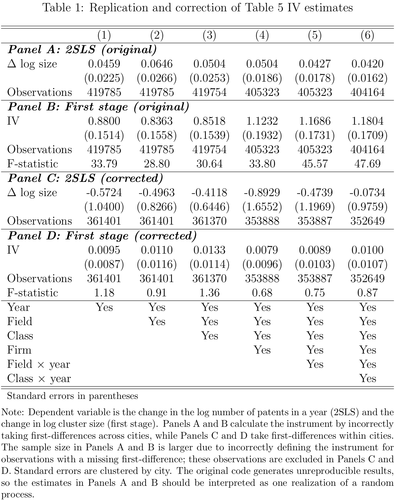
The original results are reproduced in Panels A and B of Table 1, and the results using the corrected instrument are in Panels C and D. Since Moretti’s results are not reproducible, my reproductions are similar but not identical to the original estimates in Table 5.⁸ The results using the corrected instrument are markedly different, however. The 2SLS estimates are now negative and nonsignificant, likely due to the first stage now being close to zero with an F-statistic around 1.⁹ Without a first stage, the IV strategy does not work. This is not evidence against agglomeration effects, but it does mean that Moretti fails to provide evidence against confounding from city-field-year shocks, such as local field-specific subsidies that affect both patenting and cluster size.

Conclusion

I reanalyze Moretti (2021) using the original data and code, and find that the results from the event study and instrumental variables regressions are caused by coding errors. The event study does not interact the treatment variable with a time indicator for the year of the treatment, and the instrument is calculated incorrectly by taking first-differences across cities. While the OLS results for agglomeration effects remain valid, they are vulnerable to confounding from sorting and omitted variable bias.