Dropping 1% of the data kills false positives

How robust are false positives to dropping 1% of your sample? Turns out, not at all.

Rachael Meager and co-authors have a paper with a new robustness metric based on dropping a small fraction of the sample. It’s called the Approximate Maximum Influence Perturbation (AMIP). Basically, their algorithm finds the observations that, when dropped, have the biggest influence on an estimate. It calculates the smallest fraction required to change an estimate’s significance, sign, and both significance and sign. In other words, if you have a significant positive result, it calculates the minimum fractions of data you need to drop in order to (1) kill significance, (2) get a negative result, and (3) get a significant negative result. The intuition here is to check whether there are influential observations that are driving a result.¹ And influence is related to the signal-to-noise ratio, where the signal is the true effect size and the noise is the relative variance of the residuals and the regressors.

In a previous post, I explored how p-hacked false positives can be robust to control variables. In this post, I want to see how p-hacked results fare under this new robustness test.

Robustness of true effects

First, let’s show that real effects are robust to dropping data. I generate data according to:

\[\tag{1} y_{i} = \beta X_{i} + \varepsilon_{i},\]

where \(X\) and \(\varepsilon\) are each distributed \(N(0,1)\). I then apply the AMIP algorithm. I repeat this process for different values of \(\beta\), and the results are shown in Figure 1.

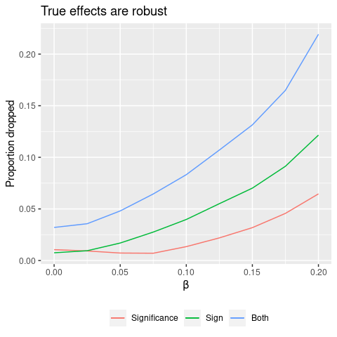
We see that as the effect size increases, the fraction of data needed to be dropped in order to flip a condition also increases. When \(\beta=0.2\), we need to drop more than 5% of the data to kill significance. This makes sense, because the true effect size increases the signal and hence the signal-to-noise ratio.

Robustness of p-hacked results

Next let’s see how robust a p-hacked result is. Now I use data

\[\tag{2} y_{i} = \sum_{k=1}^{K} \beta_{k} X_{k,i} + \gamma z_{i} + \varepsilon_{i}.\]

We have \(K\) potential treatment variables, \(X_{1,i}\) to \(X_{K,i}\), and a control variable \(z_{i}\). I draw \(X_{k,i}\), \(z_{i}\), and \(\varepsilon_{i}\) from \(N(0,1)\). I set \(\beta_{k}=0\) for all \(k\), so that \(X_{k}\) has no effect on \(y\), and the true model is

\[\tag{3} y_{i} = \gamma z_{i} + \varepsilon_{i}.\]

I’m going to p-hack using the \(X_{k}\)’s, running \(K=20\) univariate regressions of \(y\) on \(X_{k}\) and selecting the one with the smallest p-value. Then I run the AMIP algorithm to calculate the fraction of data needed to kill significance, etc.

In my previous post on p-hacking, we learned that when \(\gamma\) is small, the partial-\(R^{2}(z)\) is small, and controlling for \(z\) is not able to kill coincidental false positives. To see whether dropping data is a better robustness check, I repeat the above process for different values of \(\gamma\).

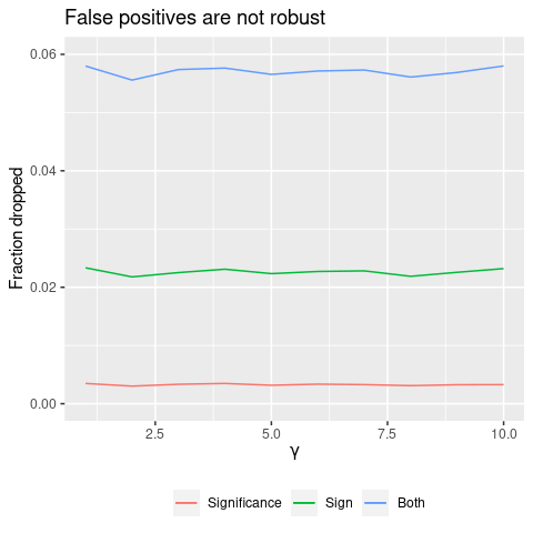
The results are in Figure 2. First, notice that we lose significance after dropping a tiny fraction of the data: about 0.3%. For \(N=1000\), that means 3 observations are driving significance.

Second, we see that the fraction dropped doesn’t vary with \(\gamma\) at all. This is good news: previously, we saw that control variables only kill false positives when they have high partial-\(R^{2}\). But dropping influential observations is equally effective for any value of \(\gamma\). So dropping data is an effective robustness check where control variables fail.

Overall, dropping data looks like an effective robustness check against coincidental false positives. Hopefully this metric becomes a widely used robustness check, and will help root out bad research.

---

Update (Nov. 5, 2021): Ryan Giordano gives a formal explanation here.

---

Footnotes

See here for R code.