Economists want to show that our results are robust, like in Table 1 below: Column 1 contains the baseline model, with no covariates, and Column 2 controls for \(z\). Because the coefficient on \(X\) is stable and significant across columns, we say that our result is robust.

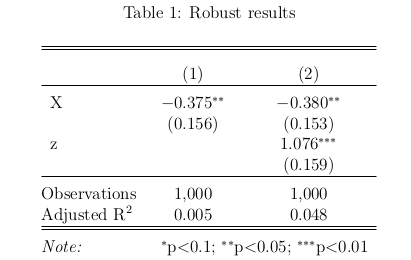
The twist: I p-hacked this result, using data where the true effect of \(X\) is zero.

In this post, I show that it can be easy to p-hack a robust result like this. Here’s the basic idea: first, p-hack a significant result by running regressions with many different treatment variables, where the true treatment effects are all zero. For 20 regressions, we expect to get one false positive: a result with \(p<0.05\). Then, using this significant treatment variable, run a second regression including a control variable, to see whether the result is robust to controls.

It turns out that the key to p-hacking robust results is to use control variables that have a low partial-\(R^{2}\). These variables don’t have much influence on our main coefficient when excluded from the regression, and also have little influence when included. In contrast, controls with high partial-\(R^{2}\) are more likely to kill a false positive. Lesson: high partial-\(R^{2}\) controls are an effective robustness check against false positives.

Setup

Let’s see how this works. Consider data for \(i=1, ..., N\) observations generated according to

\[\tag{1} y_{i} = \sum_{k=1}^{K} \beta_{k} X_{k,i} + \gamma z_{i} + \varepsilon_{i}.\]

We have \(K\) potential treatment variables, \(X_{1,i}\) to \(X_{K,i}\), and a control variable \(z_{i}\). I draw \(X_{k,i} \sim N(0,1)\), \(z_{i} \sim N(0,1)\), and \(\varepsilon_{i} \sim N(0,1)\), so that \(X_{k,i}\), \(z_{i}\), and \(\varepsilon_{i}\) are all independent, but could be correlated in the sample. I set \(\beta_{k}=0\) for all \(k\), so that \(X_{k}\) has no effect on \(y\), and the true model is

\[\tag{2} y_{i} = \gamma z_{i} + \varepsilon_{i}.\]

I’m going to p-hack using the \(X_{k}\)’s, running \(K\) regressions and selecting the \(k^{*}\) with the smallest p-value. I p-hack the baseline regression of \(y\) on \(X_{k}\), by running \(K\) regressions of the form

\[\tag{3} y_{i} = \alpha_{1,k} + \beta_{1,k}X_{k,i} + \nu_{i}. % kinda abusing notation here, since beta_{1,k} is not the coefficient in the DGP (beta_{k})\]

I use the ‘1’ subscript to indicate that this is the baseline model in Column 1. Out of these \(K\) regressions, I select the \(k^{*}\) with the smallest p-value on \(\beta_{1}\). That is, I select the regression

\[\tag{4} y_{i} = \alpha_{1,k^{*}} + \beta_{1,k^{*}}X_{k^{*},i} + \nu_{i}.\]

When \(K\geq 20\), we expect \(\hat{\beta}_{1,k^{*}}\) to have \(p<0.05\), since with a 5% significance level (i.e., false positive rate), the average number of significant results is \(20\times0.05 = 1\). This is our p-hacked false positive.

To get a robust sequence of regressions, I need my full model including \(z\) to also have a significant coefficient on \(X_{k^{*},i}\). To test this, I run my Column 2 regression:

\[\tag{5} y_{i} = \alpha_{2,k^{*}} + \beta_{2,k^{*}}X_{k^{*},i} + \gamma z_{i} + \varepsilon_{i}.\]

Given that we p-hacked a significant \(\hat{\beta}_{1,k^{*}}\), will \(\hat{\beta}_{2,k^{*}}\) also be significant?

Homogeneous \(\beta=0\)

First, I show a case where p-hacked results are not robust. I use the data-generating process from above with \(\beta=0\).

When regressing \(y\) on \(X_{k}\) in the p-hacking step, we have

\[\tag{6} y_{i} = \alpha_{1,k} + \beta_{1,k} X_{k,i} + \nu_{i},\]

where

\[\tag{7} \begin{align} \nu_{i} &= \sum_{j \neq k}^{K} \beta_{1,j} X_{j,i} + \gamma z_{i} + \varepsilon_{i} \\ &= \gamma z_{i} + \varepsilon_{i}. \end{align}\]

We estimate the slope coefficient as

\[\tag{8} \hat{\beta}_{1,k} = \frac{\widehat{Cov}(X_{k},y)}{\widehat{Var}(X_{k})} = \frac{\gamma \widehat{Cov}(X_{k},z) + \widehat{Cov}(X_{k},\varepsilon)}{\widehat{Var}(X_{k})}.\]

Since \(\beta=0\), we should only find a significant \(\hat{\beta}_{1,k}\) due to a correlation between \(X_{k}\) and the components of the error term \(\nu_{i}\): (1) \(\gamma \widehat{Cov}(X_{k},z)\), and (2) \(\widehat{Cov}(X_{k},\varepsilon)\).

When \(\gamma \widehat{Cov}(X_{k},z)\) is the primary driver of \(\hat{\beta}_{1,k}\), controlling for \(z\) in Column 2 will kill the false positive.

Turning to the full regression in Column 2, we get

\[\begin{align} \tag{9} \hat{\beta}_{2,k} &= \frac{\widehat{Cov}(\hat{u},y)}{\widehat{Var}(\hat{u})} = \frac{\widehat{Cov}((X_{k} - \hat{\lambda}_{1} z),\varepsilon)}{\widehat{Var}(\hat{u})} \\ &= \frac{\widehat{Cov}(X_{k},\varepsilon) - \hat{\lambda}_{1} \widehat{Cov}(z,\varepsilon)}{\widehat{Var}(\hat{u})}. \end{align}\]

This is from the two-step Frisch-Waugh-Lovell method, where we first regress \(X_{k}\) on \(z\) (\(X_{k} = \lambda_{0} + \lambda_{1} z + u\)) and take the residual \(\hat{u} = X_{k} - \hat{\lambda}_{0} - \hat{\lambda}_{1} z\). Then we regress \(y\) on \(\hat{u}\), using the variation in \(X_{k}\) that’s not due to \(z\), and the resulting slope coefficient is \(\hat{\beta}_{2,k}\).¹ We can see that controlling for \(z\) literally removes the \(\gamma \widehat{Cov}(X_{k},z)\) term from our estimate.

Hence, to p-hack robust results, we want \(\hat{\beta}_{1,k}\) to be driven by \(\widehat{Cov}(X_{k},\varepsilon)\), since that term is also in \(\hat{\beta}_{2,k}\). If we have a significant result that’s not driven by \(z\), then controlling for \(z\) won’t affect our significance.

Simulations

Setting \(K=20, N=1000\), and \(\gamma=1\), I perform \(1000\) replications of the above procedure: I run 20 regressions, select the most significant \(X_{k^{*}}\) and record the p-value on \(\hat{\beta}_{1,k^{*}}\), then add \(z\) to the regression and record the p-value on \(\hat{\beta}_{2,k^{*}}\). As expected when using a \(5\%\) significance level, I find that out of the \(K\) regressions in the p-hacking step, the average number of significant results is \(0.05\). I find that \(\hat{\beta}_{1,k^{*}}\) is significant in 663 simulations (=66%). But only 245 simulations (=25%) have both a significant \(\hat{\beta}_{1,k^{*}}\) and a significant \(\hat{\beta}_{2,k^{*}}\), meaning that only 37% (=245/663) of p-hacked Column 1 results have a significant Column 2. So in the \(\beta=0\) case, we infer that \(\widehat{Cov}(X_{k},\varepsilon)\) is small relative to \(\gamma \widehat{Cov}(X_{k},z)\). With these parameters, it’s not easy to p-hack robust results.

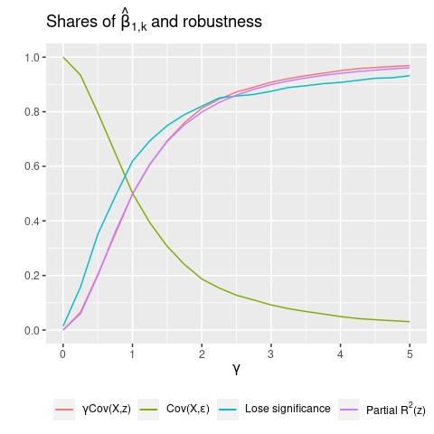
Figure 1 repeats this process for a range of \(\gamma\)’s. I plot the shares of \(\gamma \widehat{Cov}(X_{k},z)\) and \(\widehat{Cov}(X_{k},\varepsilon)\) in \(\hat{\beta}_{1,k}\).² We see that when \(\gamma=0\), \(\gamma \widehat{Cov}(X_{k},z)\) has 0 weight, but its share increases quickly. Closely correlated with this share is the fraction of significant results losing significance after controlling for \(z\). Specifically, this is the fraction of simulations with a nonsignificant \(\hat{\beta}_{2,k}\), out of the simulations with a significant \(\hat{\beta}_{1,k}\). And even more tightly correlated with \(\gamma \widehat{Cov}(X_{k},z)\) is the partial \(R^{2}\) of \(z\).³ Intuitively, as \(\gamma\) increases, the additional improvement in model fit from adding \(z\) also increases, which by definition increases \(R^{2}(z)\). Hence, \(R^{2}(z)\) turns out to be a useful proxy for the share of \(\gamma \widehat{Cov}(X_{k,i},z_{i})\), which we can’t calculate in practice. Lesson: when partial-\(R^{2}(z)\) is large, controlling for \(z\) is an effective robustness check for false positives. This is because a large \(\gamma \widehat{Cov}(X_{k},z)\) implies both (1) a large \(R^{2}(z)\); and (2) that \(z\) is more likely to be the source of the false positive, and hence controlling for \(z\) will kill it. So now we have a new justification for including control variables, apart from addressing confounders: to rule out false positives driven by coincidental sample correlations.

Heterogeneous \(\beta_{i} \sim N(0,1)\)

However, you might think that \(\beta=0\) is not a realistic assumption. As Gelman says: “anything that plausibly could have an effect will not have an effect that is exactly zero.” So let’s consider the case of heterogeneous \(\beta_{i}\), where each individual \(i\) has their own effect drawn from \(N(0,1)\). For large \(N\), the average effect of \(X\) on \(y\) will be 0, but this effect will vary by individual. This is a more plausible assumption than \(\beta\) being uniformly 0 for everyone. And as we’ll see, this also helps for p-hacking, by increasing the variance of the error term.

Here we have data generated according to

\[\tag{10} y_{i} = \sum_{k=1}^{K} \beta_{k,i} X_{k,i} + \gamma z_{i} + \varepsilon_{i},\]

where \(\beta_{k,i} \sim N(0,1)\).

Then, when regressing \(y\) on \(X_{k}\), we have

\[\tag{11} y_{i} = \alpha_{1,k} + \delta_{1,k} X_{k,i} + v_{i},\]

where

\[\tag{12} v_{i} = -\delta_{1,k} X_{k,i} + \beta_{k,i} X_{k,i} + \sum_{j \neq k}^{K} \beta_{j,i} X_{j,i} + \gamma z + \varepsilon_{i}.\]

When effects are heterogeneous (i.e., we have \(\beta_{k,i}\) varying with \(i\)), a regression model with a constant slope \(\delta_{1,k}\) is misspecified. To emphasize this, I include \(-\delta_{1,k} X_{k,i}\) in the error term.⁴

The estimated slope coefficient is

\[\tag{13} \begin{align} \hat{\delta}_{1,k} &= \frac{\widehat{Cov}(X_{k,i},y_{i})}{\widehat{Var}(X_{k,i})} \\ &= \frac{\sum_{j=1}^{K} \widehat{Cov}(X_{k,i},\beta_{j,i}X_{j,i}) + \gamma \widehat{Cov}(X_{k,i},z_{i}) + \widehat{Cov}(X_{k,i},\varepsilon)_{i}}{\widehat{Var}(X_{k,i})} \end{align}\]

From Aronow and Samii (2015), we know that the slope coefficient converges to a weighted average of the \(\beta_{k,i}\)’s:

\[\tag{14} \hat{\delta}_{1,k} \rightarrow \frac{E[w_{i} \beta_{k,i}]}{E[w_{i}]},\]

where \(w_{i}\) are the regression weights: the residuals from regressing \(X_{k}\) on the other controls. In this case, as we’re using a univariate regression, the residuals are simply demeaned \(X_{k}\) (when regressing \(X\) on a constant, the fitted value is \(\bar{X}\)).

Because \(\beta_{k,i} \sim N(0,1)\), we have \(E[w_{i} \beta_{k,i}]=0\) and hence \(\hat{\delta}_{1,k}\) converges to 0. So any statistically significant \(\hat{\delta}_{1,k}\) that we estimate will be a false positive.

There are three terms that make up \(\hat{\delta}_{1,k}\) and could drive a false positive: (1) \(\sum_{j=1}^{K} \widehat{Cov}(X_{k,i},\beta_{j,i}X_{j,i})\), (2) \(\gamma \widehat{Cov}(X_{k},z)\), and (3) \(\widehat{Cov}(X_{k},\varepsilon)\).

Now we have a new source of false positives, case (1), due to heterogeneity in \(\beta_{k,i}\). Note that controlling for \(z\) will only affect one out of three possible drivers, so now we should expect our false positives to be more robust to control variables, compared to when \(\beta=0\). To see this, note that when controlling for \(z\) in the full regression, we have

\[\tag{15} \begin{align} \hat{\delta}_{2,k} &= \frac{\widehat{Cov}(\hat{u}_{i},y_{i})}{\widehat{Var}(\hat{u}_{i})} \\ &= \frac{\sum_{j=1}^{K} \widehat{Cov}(X_{k,i} - \hat{\lambda}_{1} z_{i},\beta_{j,i}X_{j,i}) + \widehat{Cov}(X_{k,i} - \hat{\lambda}_{1} z_{i},\varepsilon_{i})}{\widehat{Var}(\hat{u}_{i})} \\ &= \frac{\sum_{j=1}^{K} \widehat{Cov}(X_{k,i},\beta_{j,i}X_{j,i}) + \widehat{Cov}(X_{k,i},\varepsilon_{i})}{\widehat{Var}(\hat{u_{i}})} \\ &- \hat{\lambda}_{1} \frac{\left[ \sum_{j=1}^{K} \widehat{Cov}(z_{i},\beta_{j,i}X_{j,i}) + \widehat{Cov}(z_{i},\varepsilon_{i}) \right] }{\widehat{Var}(\hat{u_{i}})} \end{align}\]

Here \(\hat{u}\) is the residual from a regression of \(X_{k}\) on \(z\): \(X_{k} = \lambda_{0} + \lambda_{1} z + u\). We obtain \(\hat{\delta}_{2,k}\) by regressing \(y\) on \(\hat{u}\), via FWL, and using the variation in \(X_{k}\) that’s not due to \(z\).

Comparing \(\hat{\delta}_{1,k}\) to \(\hat{\delta}_{2,k}\), we see that \(\sum_{j=1}^{K} \widehat{Cov}(X_{k,i},\beta_{j,i}X_{j,i}) + \widehat{Cov}(X_{k_{i}},\varepsilon_{i})\) shows up in both estimates. Hence, if our p-hacking selects for a \(\hat{\delta}_{1,k}\) with a large value of these terms, we’re also selecting for the majority of the components of \(\hat{\delta}_{2,k}\). In contrast to the \(\beta=0\) case, now we should expect \(\gamma \widehat{Cov}(X_{k,i},z_{i})\) to be dominated, and significance in Column 1 should carry over to Column 2.

Simulations

I repeat the same procedure as before, running \(K=20\) regressions of \(y\) on \(X_{k}\) and \(z\), taking the \(X_{k}\) with the smallest p-value, \(X_{k^{*}}\), and then running another regression while excluding \(z\). Again, I use \(\gamma=1\) and perform \(1000\) replications. Here I use robust standard errors to address heteroskedasticity.

I find that \(\hat{\delta}_{1,k^{*}}\) is significant in 650 simulations (=65%). But this time, 569 simulations (=57%) have both a significant \(\hat{\delta}_{1,k^{*}}\) and a significant \(\hat{\delta}_{2,k^{*}}\). So 88% (=569/650) of p-hacked Column 1 estimates also have a significant Column 2. Compare this to 37% in the \(\beta=0\) case. That’s what I call p-hacking a robust result! We infer that \(\gamma \widehat{Cov}(X_{k,i},z_{i})\) is too small relative to the other components for its presence or absence to affect our estimates very much.

To illustrate how \(\hat{\delta}_{1,k}\) is determined, I plot the shares of its three constituent terms while varying \(\gamma\).⁵

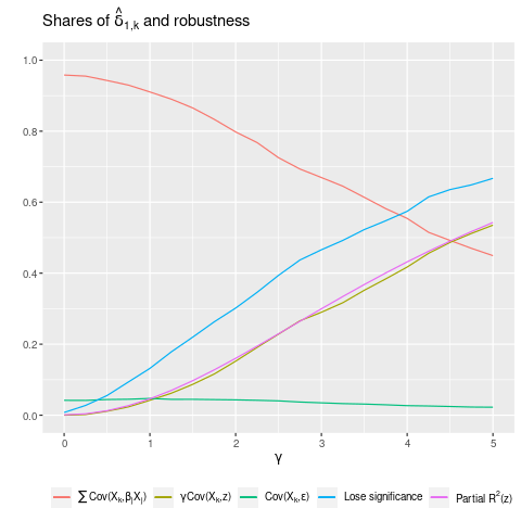
As shown in Figure 2, when \(\gamma\) is small, most of the weight in \(\hat{\delta}_{1,k}\) is from \(\sum_{j=1}^{K} \widehat{Cov}(X_{k,i},\beta_{j,i}X_{j,i})\), indicating that its \(K\) terms provide ample opportunity for correlations with \(X_{k^{*},i}\). But as \(\gamma\) increases, this share falls, while the share of \(\gamma \widehat{Cov}(X_{k,i},z_{i})\) rises linearly. The share of \(\widehat{Cov}(X_{k,i},\varepsilon_{i})\) is small and decreases slightly. Looking at robustness, we see that the fraction of significant results losing significance rises much more slowly than in the \(\beta=0\) case. And we again see a tight link between partial-\(R^{2}(z)\) and the share of \(z\) in \(\hat{\delta}_{1,k}\).⁶

Overall, we can see why controlling for \(z\) is less effective with heterogeneous effects: \(\hat{\delta}_{1,k}\) is mostly not determined by \(\gamma \widehat{Cov}(X_{k,i},z_{i})\), so removing it (by controlling for \(z\)) has little effect. In other words, when variables have low partial-\(R^{2}\), controlling for them won’t affect false positives.

Conclusion

In general, economists think about robustness in terms of addressing potential confounders. I haven’t seen any discussion of robustness to false positives based on coincidental sample correlations. This is possibly because it seems hopeless: we always have a 5% false positive rate, after all. But as I’ve shown, adding high partial-\(R^{2}\) controls is an effective robustness check against p-hacked false positives.⁷ So we have a new weapon to combat false positives: checking whether a result remains significant as high partial-\(R^{2}\) controls are added to the model.

Footnotes

See here for R code. Click here for a pdf version of this post.