In the last post I used continuous quantities of housing: people could buy, say, 1.26 homes. Here I show how a supply and demand model works with discrete quantities, and with a unit demand constraint, where people buy at most one unit of housing. This involves a different than the perfect substitutes case, but we arrive at the same conclusion regarding vacancy chains, demand cascades, and yuppie fishtanks.

A supply and demand equilibrium

Consumers start with a willingness to pay for Old and New apartments. They buy the housing type with the largest difference between valuation and price: \(v-p\). To satisfy the unit demand constraint, their demand only counts in the market of the type they choose. So one rich person could buy up all of the homes, but the unit demand constraint prevents this, by requiring them to buy their highest-valued type, and removing their demand for the other types. Here, there are five consumers, and everyone value New apartments more than Old.

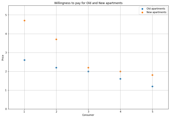
I’ll show an initial equilibrium where Person 1 buys a New apartment, and Persons 2 and 3 buy Old. Because Person 1 buys New, their demand is removed from the Old market. Hence, the aggregate demand curve for Old apartments looks like this:

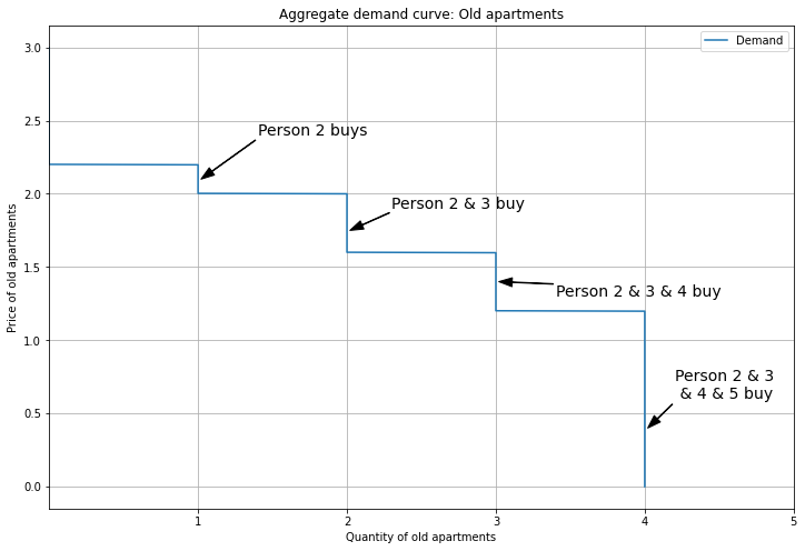
Since each person demands one unit, aggregate demand tops out at four. Next, here’s the supply and demand equilibrium for Old apartments. The supply curve is vertical, representing a fixed stock of Old apartments. Since the supply curve overlaps the demand curve for some segment, technically the equilibrium is not well-defined. However, this is not a big deal, because we can pretend the supply curve is slightly sloping upward, so the intersection is unique (though this brings in continuous quantities). Alternatively, if we had a large number of consumers, the demand curve would be a straight line that intersects supply uniquely; working with discrete quantities is just a pain.

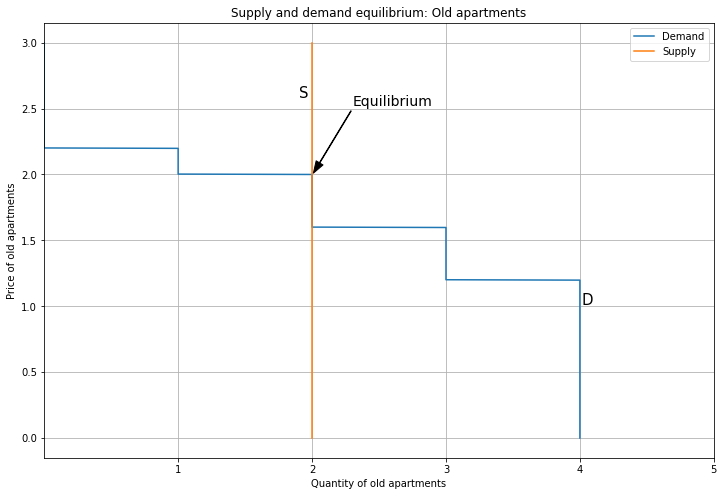
So Persons 2 and 3 each get an Old apartment, and the price is 2. Note that Persons 4 and 5 are initially priced-out, and don’t get a home. We can interpret this as having to move away, or living in their car (or being homeless).

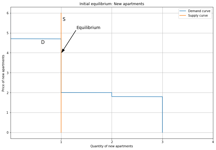
Next we have the aggregate demand curve for New apartments. Here we show Persons 1, 4, and 5, because Persons 2 and 3 buy Old apartments, so their demand for New is removed (by the unit demand constraint).

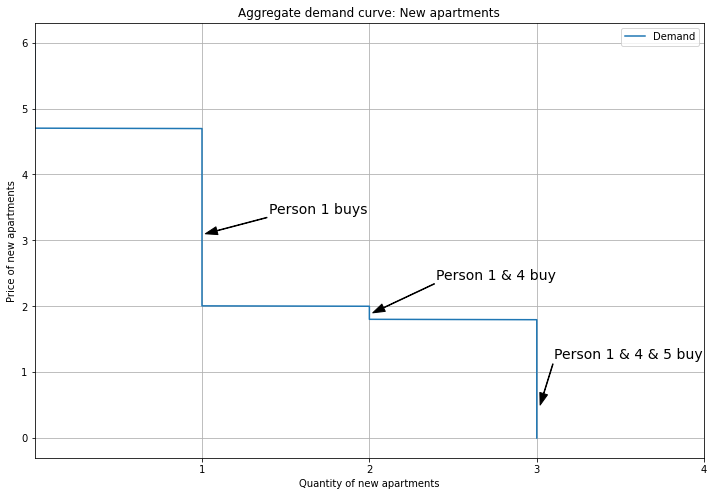
In the initial equilibrium, only Person 1 gets a new apartment, and the price is 4. The supply curve is vertical, representing zoning constraints: developers cannot build any more, even if prices went up. Note that Persons 4 and 5 are priced out here as well.

Vacancy chains

To show a vacancy chain, we increase the supply of New apartments. This will allow Person 2 to upgrade, vacating their Old apartment, which in turn allows Person 4 to get a home (instead of being homeless).

The higher supply of New apartments reduces the price, as we move down the demand curve. This lower price induces Person 2 to re-evaluate their housing choice. Their willingness to pay is 3.7 for New apartments, and 2.2 for Old. The price for New apartments was 4, so they chose Old. But now the price is 2, so their payoff for a New apartment is 3.7 - 2 = 1.7, and the payoff for an Old apartment is 2.2 - 2 = 0.2 Hence, the New apartment is a better deal, so they switch markets from Old to New.

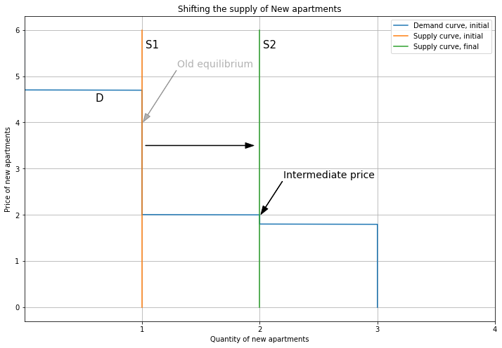
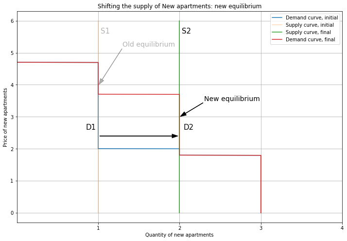
Person 2 upgrading means that we also change which market their demand contributes to. So we subtract their demand from the Old demand curve, and add it to the New demand curve, shifting it to the right. For New apartments, this pushes up the price. Note that we can end up out of equilibrium if this increase in price is not consistent with Person 2’s willingness to pay. Here, I’ll use the modelling flexibility we have from the supply and demand curve overlapping to choose a new equilibrium price of 3.

Since Person 2 upgrades, we remove their demand for Old apartments, shifting it left. Now Persons 3 and 4 are able to get an Old apartment, and the price falls to 1.6. (That is, supply intersects demand on the section of the demand curve where Persons 3 and 4 buy.) This is the vacancy chain in action: Person 4 was initially priced out and didn’t have a home, but by adding a New apartment, we have freed up an Old apartment for Person 4 to live in!

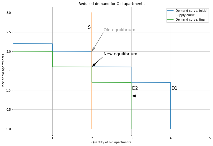
To make sure this is an equilibrium, let’s check the payoffs. Person 1 is happy to buy New, because they get 4.7 - 3 = 1.7 from New and 2.6 = 1.6 = 1 from Old. Person 2’s payoffs are 3.7 - 3 = 0.7 (New) and 2.2 - 1.6 = 0.6, so they buy New. Person 3 gets 2.2 - 3 < 0 for New and 2 - 1.6 = 0.4 from Old, so they buy Old. So each consumer’s choice is consistent, hence, these prices define an equilibrium.

Note that with unit demand, we are able to have consumers being priced out (like Person 4 initially). With continuous quantities, this was not possible, since they could always buy some infinitesimal quantity, and so can’t be priced out completely. But with discrete units, Person 4 initially doesn’t get anything, then thanks to the vacancy chain, they get an Old apartment.

Demand cascade and yuppie fishtank

Now let’s see how demand cascades and yuppie fishtanks work in the unit demand case. Since people can be priced out entirely, demand cascades will push people out of old apartments, and yuppie fishtanks will allow them to avoid being pushed out.

We’ll use the same willingness to pay as before, but this time we’ll start with Person 1 living outside of the city. Person 2 starts in a New apartment, so they don’t contribute to demand for Old apartments. That leaves Persons 3, 4, and 5 making up the aggregate demand curve for Old apartments.

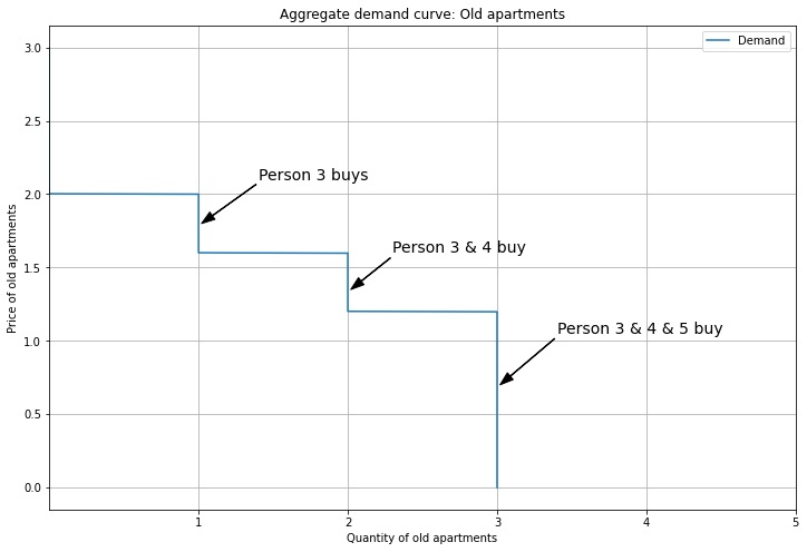
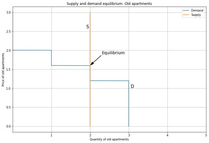
There are two Old units, so the equilibrium has Person 3 and 4 each getting an Old unit at a price of 1.6.

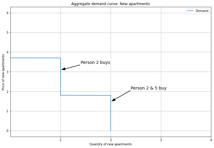
For New apartments, Persons 2 and 5 contribute to the demand curve.

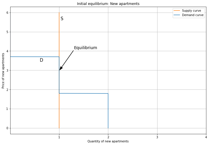
But there’s only one New unit supplied, so only Person 2 gets a New unit in the equilibrium. The price is 3, which ensures that everyone is choosing their best option. Person 5 is priced out of both housing types, and has to live in their car.

The demand cascade starts with Person 1 moving in and bidding for a New apartment. This shifts the demand curve to the right (from D1 to D2a), increasing the price from 3 to 4.

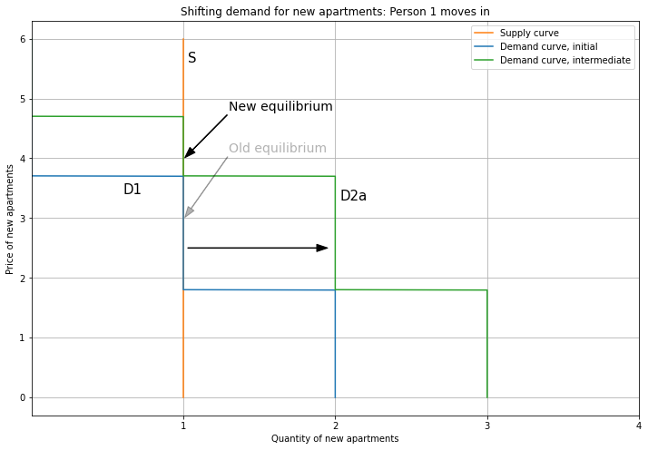
Since Person 1 is richer, they outbid Person 2 for the New apartment, so now Person 2 downgrades to an Old apartment. Hence, we remove their demand from the New demand curve; this does not affect the new equilibrium. Now only Persons 1 and 5 contribute to the aggregate demand curve.

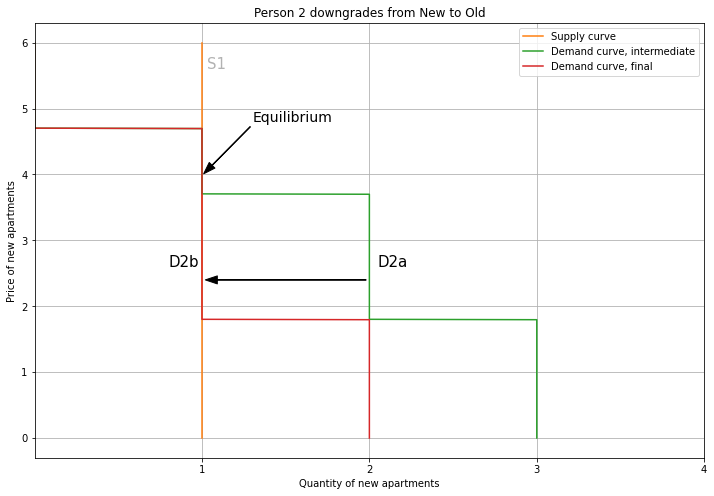
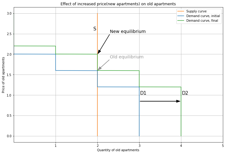
Turning to Old market, we add in Person 2’s demand, shifting the demand curve to the right. This pushes up the price, from 1.6 to 2. Now Persons 2 and 3 get an Old apartment, and Person 4 is priced out and doesn’t have a home. This is the demand cascade: when high-income Person 1 moves in, they bid up the price of new apartments, leading Person 2 to downgrade to an old apartment, which leaves Person 4 being priced out. In short, when supply is restricted, rich people moving in forces poor people to move out.

But what if supply is not restricted, and grows to match the increase in demand? This is the yuppie fishtank: by building a new glass tower to contain Person 1, we absorb their demand and protect the old apartments from competition. So we shift supply from 1 to 2, reducing the price.

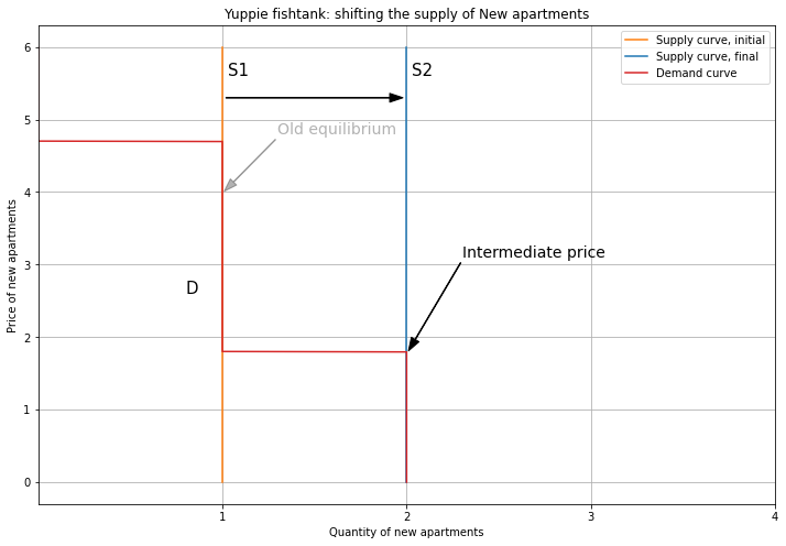
This lower price induces Person 2 to upgrade back to a New apartment. So the demand curve shifts right, and the price is 3. This is the same as the initial equilibrium: the yuppie fishtank has absorbed Person 1’s demand, keeping prices flat.

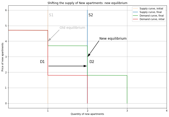
And since Person 2 is not competing for an Old apartment, the demand curve shifts left. Thanks to the yuppie fishtank, Person 4 gets to stay in their Old unit, and isn’t priced out.

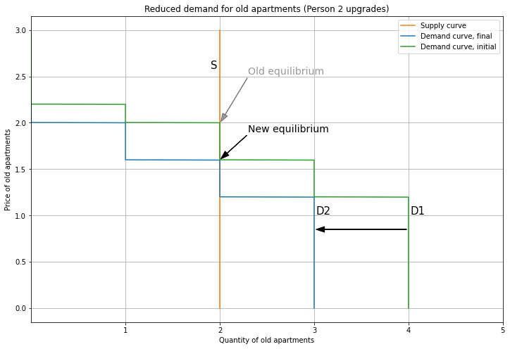
Notice that a yuppie fishtank can cancel out a demand cascade caused by a rich newcomer, while a vacancy chain triggered by a rich local upgrading is an inverse demand cascade.

---

See here and here for code to produce the graphs.