When we upzone land from single-family zoning to apartment zoning, we change the allocation of a city’s fixed stock of land. Upzoning makes apartment-zoned land more abundant and hence cheaper, while single-family-zoned land becomes scarcer and more expensive. Because land is an input into the production of housing, upzoning reduces the cost of building apartments, and hence is a key policy option for reducing housing costs.

In this post I’ll set up a two-sector model of land and show the effects of upzoning. (If you get stuck, try reading this post first.) House developers can use either single-family-zoned land or apartment-zoned land to produce houses, while apartment developers can use only apartment-zoned land. Since it’s more lucrative to build an apartment building than a house on a given parcel, apartment developers are willing to pay more for land; as a result, the price of apartment-zoned land is higher than the price of single-family-zoned land.

Upzoning moves a parcel from the single-family- to the apartment-zoned market. This makes apartment-zoned land more abundant, reducing its price; because land is an input into the production of apartments, upzoning reduces the price of apartments. In the extreme case, if we upzone all land, then house developers are indifferent between the two types of land, and we get an equilibrium where land prices are equal across submarkets.

A two-sector model of land

Consider a representative house developer with perfect substitutes preferences over house-zoned and apartment-zoned land. For the house developer, a parcel is a parcel, since they can build a house on it regardless of the zoning. (Parcels of different zoning types are identical in size.) Hence, they treat both types of land as interchangeable, and will choose the lower-price option. To simplify, I assume they have a fixed budget to spend; in a complete model, developer demand for the input (land) is derived from the price of the output (housing). Also note that we are considering vacant parcels with no teardown cost.

Click below to see the underlying demand functions.

Math

Let \(x_{H}\) = house-zoned land, \(x_{A}\) = apartment-zoned land. Let \(x_{i,j}\) be quantity demanded by developer type \(i\) for land type \(j\), with budget \(m_{i}\). Given perfect substitutes utility \(u(x_{H},x_{A}) = a x_{H} + b x_{A}\), we can derive the demand functions with the threshold defined by equating the marginal rate of substitution (\(a/b\)) with the price ratio (\(p_{H}/p_{A}\)). If \(p_{H}/a > p_{A}/b\), the developer chooses \(x_{H}\) and spends their entire budget on it; otherwise, they choose \(x_{A}\). Here the house developer has \(a = b = 1\).

With perfect substitutes preferences, we get a corner solution: the optimal choice is one or the other, and not a mix of both. Note that the demand functions take both \(p_{H}\) and \(p_{A}\) as arguments, so they define a 3-dimensional surface.

The apartment developer values only apartment-zoned land.

\[\begin{aligned} \begin{split} &u_{H}(x_{H},x_{A}) = x_{H} + x_{A} \\ &u_{A}(x_{H},x_{A}) = x_{A} \\ &m_{H} = 24 \\ &m_{A} = 12 \\ &x_{H,H} = \begin{cases} 0, & p_{H} > p_{A} \\ \in \left[0, \frac{m_H}{p_H} \right], & p_H = p_A \\ \frac{m_{H}}{p_{H}}, & p_{H} < p_{A} \\ \end{cases} \\ &x_{H,A} = \begin{cases} \frac{m_{H}}{p_{A}}, & p_{H} > p_{A} \\ \in \left[0, \frac{m_H}{p_A} \right], & p_H = p_A \\ 0, & p_{H} < p_{A} \\ \end{cases} \\ &x_{A,H} = 0 \\ &x_{A,A} = \frac{m_A}{p_A} \\ \end{split} \end{aligned}\]

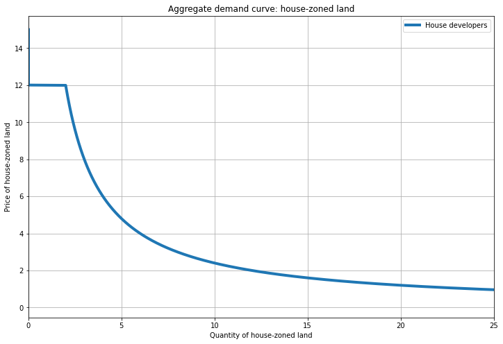
The graph below shows the demand curve for house-zoned land, with the price of of house-zoned land (\(P_H\)) on the y-axis. Recall that this is an inverse demand function, so we read it as: for a given price, what quantity of land is demanded? For example, when the price is 2, quantity demanded is 12.

Here, I’m showing an equilibrium where the price of the substitute good (apartment-zoned land) is \(P_A = 12\), so when \(P_H < 12\), the house developer buys only house-zoned land and spend their entire budget on it (bottom curved segment). The horizontal segment is where \(P_H = P_A\), so the house developer is indifferent; any quantity along this segment is equally good (and the remaining budget is spent on apartment-zoned land). When \(P_H > 12\), apartment-zoned land is cheaper, so demand for house-zoned land is 0 and the demand curve overlaps the y-axis.

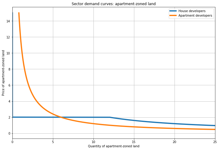
For the apartment-zoned land market, we have to aggregate the demand of both house and apartment developers (see graph below). Apartment developers spend their whole budget on apartment-zoned land, regardless of how cheap house-zoned land gets. Because they have higher willingness to pay, their quantity demanded is larger at higher prices. (Note that I’m using continuous quantities, which allows buying an infinitesimally-small quantity of land; in practice, the demand curve would intersect the y-axis at some price.)

As before, house developers will spend everything on apartment-zoned land if it is cheap enough (bottom curved segment in blue). If apartment-zoned land is more expensive than house-zoned land, the demand curve is 0 and overlaps the y-axis (and they go all-in on house-zoned land). Here, the equilibrium has the substitute price at \(P_H=2\), so when \(P_A = P_H = 2\), they are indifferent between the two, corresponding to the horizontal segment.

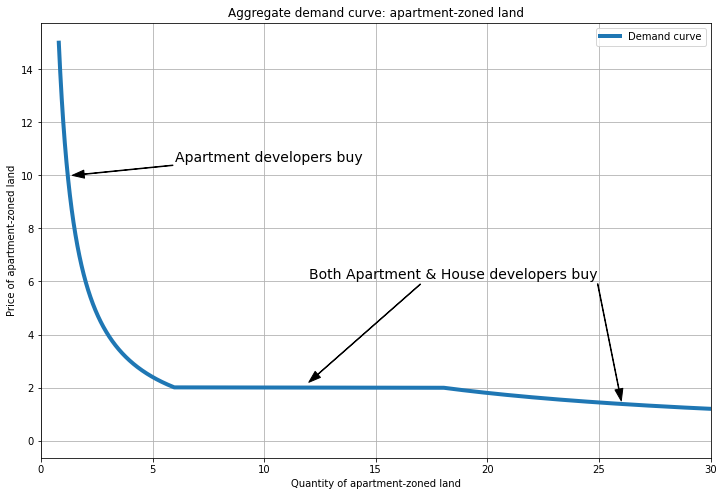
Adding up the sector demand curves horizontally, we get aggregate demand for apartment-zoned land (see below). In the upper-left curved segment we will get a corner solution where apartment developers buy only apartment-zoned land, and house developers buy only house-zoned land. (When \(P_A > 2\), the aggregate demand curve is equal to the apartment developers’ demand curve.) The horizontal segment is the interior solution where house developers buy some apartment-zoned land and prices are equal. (The bottom-right curved segment is the other corner solution where both developers buy only apartment zoned land and \(P_A < P_H\); I’ll discuss this case later.)

Here’s an equilibrium for the corner solution. To maintain incentive compatibility, we require that \(P_{A} > P_{H}\), so that the house developer chooses the cheaper option (house-zoned land). This holds when the (fixed) supply of house-zoned land is large and the supply of apartment-zoned land is small.

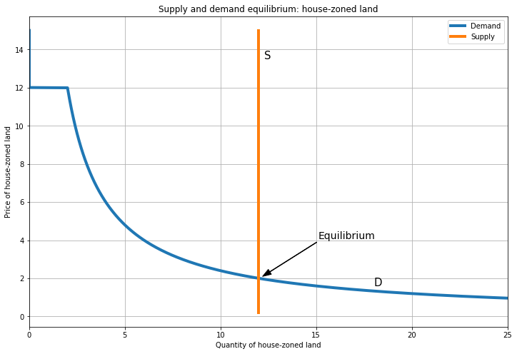
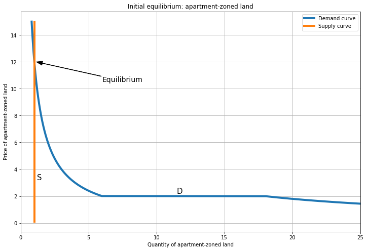
At these prices, all supply is demanded, so this is an equilibrium. Note that we also have a market clearing condition for supply across sectors: \(S_{A} + S_{H} = S = 13\), where \(S\) is the total stock of land.

Small upzoning

Let’s upzone a small amount by moving one parcel from the house market to the apartment market (so \(S_{A}\) increases from 1 to 2 and \(S_{H}\) falls from 13 to 12). This shifts \(S_{A}\) to the right, which reduces \(P_{A}\) from 12 to 6. At the same time, \(S_{H}\) shifts left, increasing \(P_{H}\) from 2 to 2.2.

Because the house developer treats the two land types as substitutes, these price changes also ‘shift’ the demand curves. (Recall from last time that this is actually a movement along the 3D demand surface.) House-zoned land becomes more expensive, so demand for its substitute (apartment-zoned land) increases; this is the shift up/right in demand for apartment-zoned land (from D1 (blue) to D2 (red)).

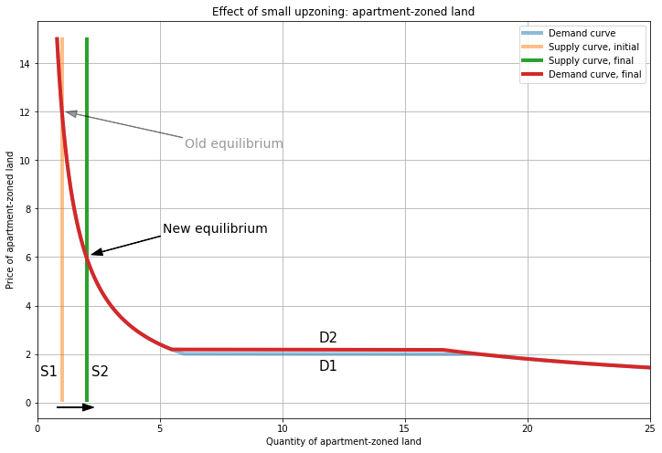
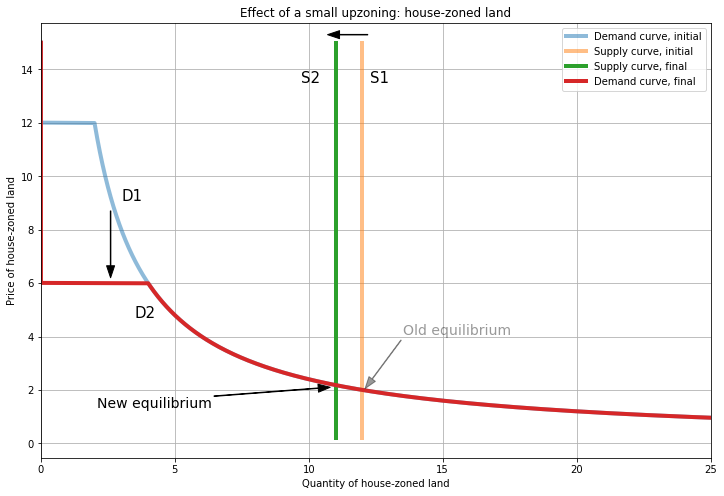
Similarly, apartment-zoned land becomes cheaper, so demand for its substitute (house-zoned land) falls, shown by the shift down/left in demand for house-zoned land. These changes in the demand curves occur away from the intersections with the supply curves, so the equilibria are unaffected.

So upzoning makes apartment-zoned land more abundant, which lessens competitive pressure among developers; this reduces the price of land, making apartments cheaper to produce. Hence, upzoning reduces the price of apartments. (The model here shows only the input market (for land), but intuitively, decreased input prices translate to decreased output prices.)

Conversely, houses become a bit more expensive, since house developers have to compete over a more limited stock of land. This is progressive, because houses are inherently more of a luxury good than apartments (ask yourself: which has more square footage, a private yard, private parking?). (Note that upzoning does not literally remove land from house developers; instead, upzoning moves land to a submarket with higher prices, where house developers are unwilling to pay the market price.)

With this model, we can see where the “but upzoning raises land costs” argument goes wrong. By changing the allocation of land across zoning types, upzoning makes apartment-zoned land cheaper and house-zoned land more expensive. While the upzoned parcel itself increases in price (from 2 to 6), that parcel was previously unavailable to apartment developers at any price. Adding it to the apartment-zoned market makes apartment developers better off, because \(P_A\) falls from 12 to 6. The fallacy in “but upzoning raises land costs” lies in looking at a single parcel instead of the market-wide price.

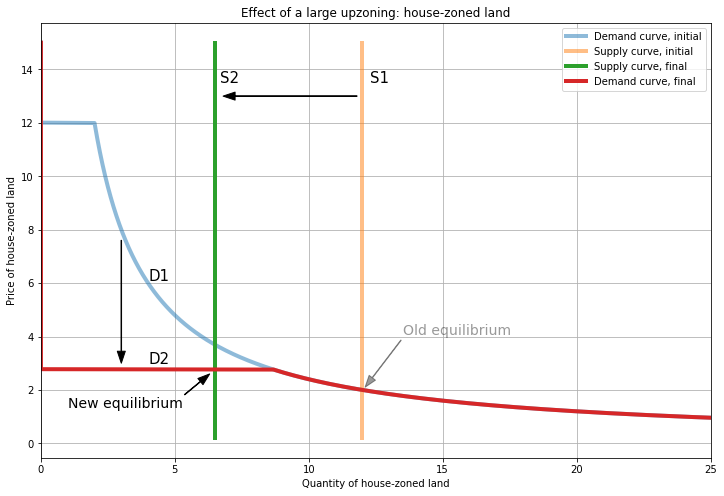
Large upzoning

Next let’s explore the interior solution where \(P_{A} = P_{H}\). Here we shift supply enough that we reach the horizontal segment of the perfect substitutes demand function. In this case, \(P_{A} = P_{H} = P \approx 2.8\); this is the maximum possible reduction in the price of apartment-zoned land. We can choose \(S_{A} \geq 4.33\) and \(S_{H} \leq 8.66\), subject to \(S_{A} + S_{H} = 13\); here I’ve used \(S_{A} = S_{H} = 6.5\).

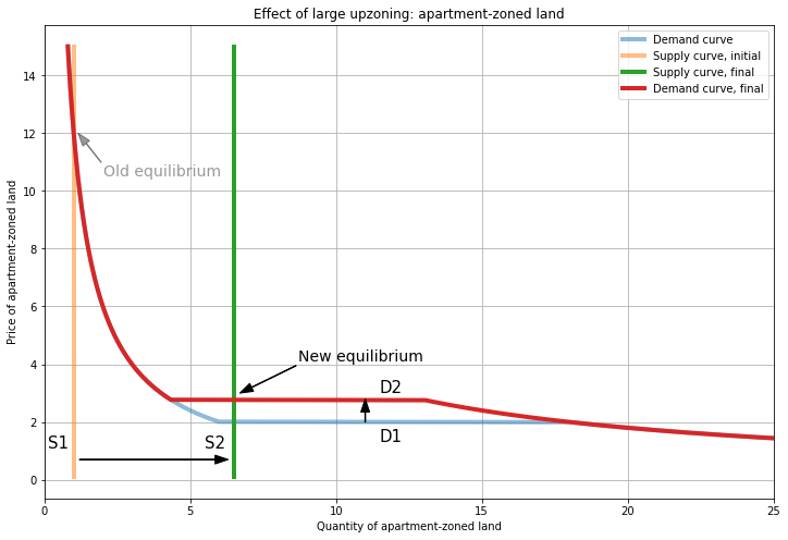
Since house developers are indifferent between the types of land, we can be anywhere on the horizontal segment as long as market clearing holds. Because the demand curve is horizontal, these movements don’t affect prices, and any allocation of supply is an equilibrium.

Maximum upzoning

Finally, let’s show the case where the entire stock of land is upzoned for apartments: \(S_{H}=0\) and \(S_{A}=S=13\). This is really the same case as the large upzoning above, because we again have \(P_{A} = P_{H} = P \approx 2.8\), and the only difference is that we move all of the way to the edge of the interior solution.

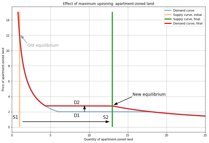
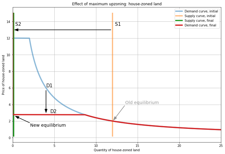
Note that this is the minimum \(P_A\) achievable, since all supply is allocated to apartment-zoned land. So when \(S\) is fixed, we can’t drive \(P_A\) down to the initial \(P_H=2\), because we have to clear the market with demand from both types of developer, whereas \(P_H=2\) comes from a market with only house developers (and hence less total demand).

When \(S_H=0\) we can also have equilibria with \(P_H > P_A\), but these have the same equilibrium price \(P_A\) and quantity \(S_A\). (With larger values of \(P_H\), the demand curve for apartment-zoned land ‘shifts’ up, but the intersection of supply and demand is unchanged.)

Discussion

A full general equilibrium model would include the output markets for houses and apartments, and show explicitly how output prices for housing are linked to input prices for land. One interesting case to look at would be where mass upzoning reduces \(P_{H}\) and hence further reduces house developers’ demand for house-zoned land. For example, a huge increase in the supply of apartments downtown induces people to move out the exurbs.

Another extension is the N-sector model with multiple types of apartments. For example, the N=3 case could have houses, 3-storey apartments, and 6-storey apartments. This would also shed light on how development feasibility changes over time. For example, as demand for houses increases, so does the price; this raises house developers’ willingness-to-pay for land. If demand from house developers is sufficiently higher than demand from 3-storey apartment developers, then no 3-storey apartments will be built.

Notice that in the small upzoning, the upzoned parcel increases in price from 2 to 6. This ‘land lift’ is the motivation for value capture policies that tax windfall gains from upzoning. But in the large upzoning, the land lift is much smaller: from 2 to 2.8. This shows the inherent tension in trying to both (a) improve housing affordability, and (b) collect taxes from new developments. Local governments are incentivized to do small spot-upzonings to maximize land lift, but because this limits the stock of apartment-zoned land, this comes at the expense of making apartments more affordable. Instead of taxing land only when it is developed, a better approach is to tax land unconditionally, like with a land value tax.

Another extension is to model anticipation effects, where landowners expect upzoning to occur in the future, which raises the price of house-zoned land today.